Multi-Physics Simulation Framework for HPM Counter-UAS Design and Evaluation

This article is a close reading of a recent defence-technology and electromagnetic-engineering paper submitted to arXiv in February 2026: “A Multi-Physics Simulation Framework for High-Power Microwave Counter-Unmanned Aerial System Design and Performance Evaluation.” The paper has been described as ushering in the era of the HPM “digital wind tunnel” — an apt analogy, since it provides a complete, reproducible simulation framework for evaluating HPM counter-UAS performance before any hardware is built. Original paper links:

• Abstract page: https://arxiv.org/abs/2602.08477

• PDF download: https://arxiv.org/pdf/2602.08477

• HTML version: https://arxiv.org/html/2602.08477v1

We now walk through the paper section by section.

[Reviewer’s note]: To be honest, the paper does not fully live up to expectations — the gap between concept and execution is larger than one might imagine. It does retain some reading value, though it does not merit a large time investment.

[Gemini commentary]

1. The sigmoid probabilistic damage model and Monte Carlo simulation are a sound choice, using probability theory to compensate for the uncertainty of physics-based modelling. In real engineering, this opens the door to fusing limited experimental data. In practice, HPM target-engagement and injection test sample sizes are usually very small, because tests are costly and damage is irreversible. How can a small amount of measured data be integrated into this framework?

1.1 Bayesian updating: fusing small-sample measured data

• Prior: Use the paper’s sigmoid theoretical model, or literature-based empirical data, as the prior probability distribution (e.g., the damage probability P_50 and slope alpha of a given chip at a given field strength).

• Likelihood: Introduce your real injection-test or field-exposure data (e.g., in 10 trials, 3 ESCs burned out at a field strength of 5 kV/m).

• Posterior calibration: Use Bayesian inference to correct the parameters of the theoretical sigmoid curve with a small amount of measured data. This preserves the trend of the physical model while giving the model the true weight of real measurements.

1.2 Building a “device–board–system” hierarchical damage mapping network

Measured data are often fragmented — some are pin-injection test data, while others are whole-system radiation test data:

• Device/board-level injection data: Correspond to the underlying thresholds of the sigmoid model (e.g., the input voltage at which CMOS latchup occurs).

• Whole-system engagement data: Correspond to the final system failure probability (e.g., drone crash or attitude loss).

• Data fusion path: Using fault tree analysis (FTA) or dynamic Bayesian networks, take board-level measured injection damage thresholds as bottom-layer inputs and propagate them up to whole-system damage. The richer your test data, the higher the certainty of these network nodes.

2. Fusing CST simulation and measured data into the Monte Carlo simulation

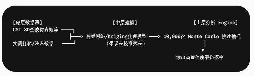
In engineering, you cannot call CST for a multi-hour full-wave computation inside each of the 10,000 Monte Carlo iterations. The correct large-scale data fusion architecture is: “offline high-fidelity computation/measurement → build a surrogate model → online Monte Carlo sampling.”

The concrete fusion implementation steps are as follows:

Paper title: A Multi-Physics Simulation Framework for High-Power Microwave Counter-Unmanned Aerial System Design and Performance Evaluation

Keywords: high-power microwave · counter-UAS · directed energy weapon · CMOS latchup · Monte Carlo simulation · electromagnetic coupling · drone neutralization

Authors: A. A. Jafari — University of Tartu, Tartu, Estonia ([email protected]); G. Anbarjafari — 3S Holding OÜ, Tartu, Estonia ([email protected])

Abstract

The proliferation of small unmanned aerial systems (sUAS) operating under autonomous guidance has created an urgent need for non-kinetic neutralization methods that are immune to conventional radio-frequency jamming. This paper presents a comprehensive multi-physics simulation framework for the design and performance evaluation of a high-power microwave (HPM) counter-UAS system operating at 2.45 GHz. The framework integrates electromagnetic propagation modelling, antenna pattern analysis, electromagnetic coupling to unshielded drone wiring harnesses, and a sigmoid-based semiconductor damage probability model calibrated to published CMOS latchup thresholds. A 10,000-trial Monte Carlo analysis incorporating stochastic variations in transmitter power, antenna pointing error, target wire orientation, polarization mismatch, and component damage thresholds yields system-level kill probabilities with 95% confidence intervals. For a baseline configuration of 25 kW continuous-wave power and a 60 cm parabolic reflector (21.2 dBi gain), the Monte Carlo simulation predicts a kill probability of 51.4±1.0% at 20 m, decreasing to 13.1±0.7% at 40 m. Pulsed operation at 500 kW peak power (1% duty cycle) extends the 90% kill range from approximately 18 m to 88 m. The framework further provides parametric design maps, safety exclusion zone calculations compliant with ICNIRP 2020 guidelines, thermal management requirements, and waveguide mode analysis. All simulation codes and results are provided for full reproducibility.

[Reviewer’s note: Really? This brings to mind a recent remark by a certain industry leader — open source saves the world!]

Introduction

The rapid proliferation of small unmanned aerial systems (sUAS) in both commercial and military domains has created asymmetric threats that challenge conventional air defence architectures [22, 26, 18, 5]. Modern consumer drones in the 250 g to 25 kg class are inexpensive, widely available, and increasingly capable of autonomous operation using pre-programmed GPS/INS waypoints or visual navigation [31, 35, 36]. In conflict zones such as Ukraine, swarms of low-cost drones have demonstrated their ability to overwhelm conventional defences, with fiber-optic guided variants rendering traditional RF jamming entirely ineffective [42, 39].

Counter-UAS (C-UAS) technologies broadly fall into kinetic (missiles, projectiles, nets) and non-kinetic (jamming, spoofing, directed energy) categories [4, 27, 21]. Kinetic solutions suffer from finite magazine depth, high cost-per-engagement, and collateral damage risk. RF jamming, while cost-effective, is fundamentally limited against autonomous drones that do not rely on a communication link [42]. High-energy laser (HEL) systems offer precision engagement but require sustained dwell time, clear atmospheric conditions, and can only engage one target at a time [1, 17].

High-power microwave (HPM) directed energy weapons offer a compelling alternative by delivering electromagnetic energy that couples directly into onboard electronic circuits, inducing semiconductor failure independent of the drone’s software architecture or communication protocol [3, 2]. Unlike jamming, HPM causes a physics-layer kill: the irreversible destruction of MOSFET gate oxides, triggering of CMOS parasitic thyristor latchup, and thermal burnout of integrated circuit junctions [12, 25, 6, 7]. Recent operational deployments of HPM C-UAS systems—notably the Epirus Leonidas, which achieved a 100% success rate against a 49-drone swarm in 2024 field testing, and the Raytheon Phaser—have validated the technology at system level [21].

Despite these advances, the open literature lacks a comprehensive, reproducible simulation framework that integrates all relevant physics—from RF source characteristics through electromagnetic propagation, coupling to target wiring, and probabilistic semiconductor damage—into a unified design tool. Prior work has addressed individual aspects: Bäckström and Lovstrand [2] compiled measured susceptibility thresholds; Nitsch et al. [23] characterized equipment-level responses; Wang et al. [30] provided SPICE-level CMOS latchup analysis; and Yu et al. [38] modelled frequency-dependent upset susceptibility. Recent studies have extended damage characterization to GaN HEMTs [28, 32, 41, 37, 33] and ESC-specific failure modes [20]. However, no prior work has synthesized these elements into a parametric design framework specifically targeting the counter-UAS application with stochastic uncertainty quantification.

This paper addresses this gap by developing a multi-physics simulation framework for HPM C-UAS system design and performance evaluation. The principal contributions are as follows:

1. A unified analytical model linking RF source parameters, antenna design, free-space propagation, and electromagnetic coupling to unshielded drone wiring to predict the induced electric field and voltage at target electronic subsystems.

2. A subsystem-resolved sigmoid damage probability model for five drone electronic subsystems (ESC, flight controller, GPS/GNSS, camera, BMS), parameterised from published experimental data.

3. A 10,000-trial Monte Carlo analysis that propagates uncertainties in transmitter power, antenna pointing, target orientation, wire geometry, and component vulnerability to produce system-level kill probabilities with confidence intervals.

4. Parametric design maps (power–aperture trade space) and safety compliance analysis against ICNIRP 2020 guidelines [24, 16].

5. Full release of all simulation source code for reproducibility.

The remainder of this paper is organized as follows. Section 2 presents the system architecture and mathematical models. Section 3 describes the simulation framework and its implementation. Section 4 presents the simulation results, including parametric analyses, Monte Carlo uncertainty quantification, and safety zone calculations. Section 5 discusses the implications, limitations, and comparison with fielded systems. Section 6 concludes the paper.

2. System Model

2.1 System architecture

The proposed HPM C-UAS system comprises six principal subsystems: (i) an AC/DC power supply unit (PSU), (ii) a high-voltage (HV) modulator providing both continuous-wave (CW) and pulsed operating modes, (iii) a cavity magnetron RF source at 2.45 GHz, (iv) a WR-340 waveguide transmission line with a ferrite circulator for source protection, (v) a parabolic reflector antenna, and (vi) a tracking subsystem incorporating an FMCW radar and an EO/IR camera on a motorized gimbal. The system-level block diagram is presented in Fig. 1.

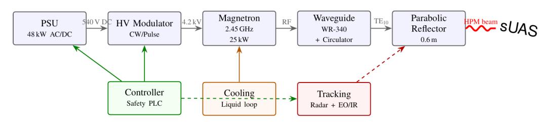
Fig. 1: Top-level schematic of the HPM C-UAS system architecture, showing the RF power chain (top), control and support subsystems (bottom), and the directed HPM beam aimed at a target sUAS.

The operating frequency of 2.45 GHz is selected for several reasons: it lies within the Industrial, Scientific and Medical (ISM) band, minimizing regulatory complexity; commodity cavity magnetrons at this frequency achieve 65–75% DC-to-RF conversion efficiency [29, 34, 19, 13]; and the corresponding wavelength λ0=c/f0=12.24 cm ensures that typical drone wiring harnesses (5–30 cm) represent a significant fraction of λ/2, maximizing electromagnetic coupling [9].

2.2 RF propagation model

The power density S at range R from a directive antenna with gain Gtx is given by the Friis transmission relation:

[Note: Want to quickly compute far-field field strength? There is a ready-made app — see our earlier article: A Practical Tool for Space Radiation Testing: Using the Field Strength Estimator to Quickly Estimate Far-Field Field Strength]

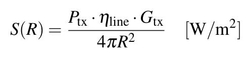
where Ptx is the transmitter output power and ηline=ηwg⋅ηfeed⋅ηradome is the aggregate transmission line efficiency. The corresponding free-space electric field magnitude is:

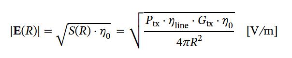
where η0=sqrt(μ0/ε0)≈377Ω is the impedance of free space. The parabolic reflector gain is:

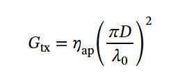
where D is the dish diameter and ηap is the aperture efficiency (taken as 0.55 for a front-fed paraboloid with standard illumination taper). The half-power (−3 dB) beamwidth is approximated as θ3dB≈70λ0/D. For the baseline configuration (D=0.60 m), this yields Gtx=21.2 dBi and θ3dB=14.3∘.

2.3 Electromagnetic coupling to target electronics

Consumer sUAS platforms are electromagnetically unshielded: flight controller PCBs, electronic speed controllers (ESCs), GPS receivers, and cameras are mounted in plastic airframes with wire harnesses acting as unintentional receiving antennas [2, 40]. The induced open-circuit voltage on a wire of physical length L illuminated by an incident electric field Einc can be modelled as a short dipole when L<λ/2:

[Reviewer’s note: The authors are starting to make idealized assumptions here, hmm.]

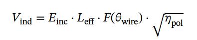
where Leff=L/2 is the effective length of a short dipole, F(θwire) accounts for the wire orientation relative to the incident polarisation, and ηpol represents the polarisation mismatch efficiency. Near the half-wave resonance (L≈λ0/2=6.12 cm), the coupling is enhanced by the antenna quality factor Q, modelled as a Gaussian resonance peak [9]:

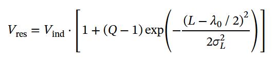
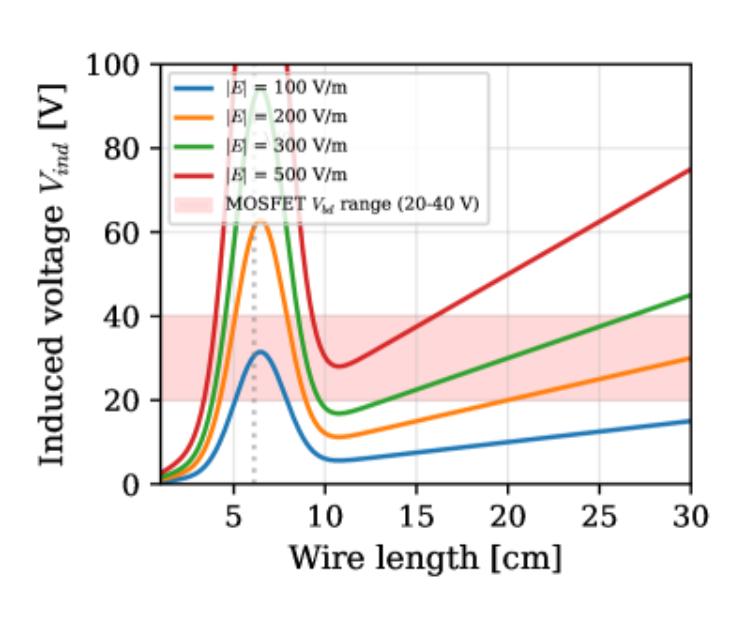
with Q≈10 and σL=0.02 m for typical unshielded harnesses. This resonance-enhanced coupling model predicts that wires in the 5–8 cm range (common for ESC signal harnesses) experience 5–10× greater induced voltage than wires of other lengths at 2.45 GHz.

[Reviewer’s note: If any expert here has run actual simulations, please comment below: how large is the gap between this theoretical calculation, CST simulation, and real-world testing? Thanks!]

2.4 Semiconductor damage probability model

The probability of damage to a semiconductor subsystem exposed to an electric field of magnitude |E| is modelled by a sigmoid (logistic) function [2, 12]:

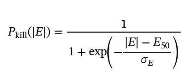
where E50 is the electric field intensity at which the damage probability equals 50%, and σE controls the steepness of the transition. This functional form is well-established in electromagnetic susceptibility analysis and captures the stochastic variability in device manufacturing, operating state, and coupling efficiency [2, 23].

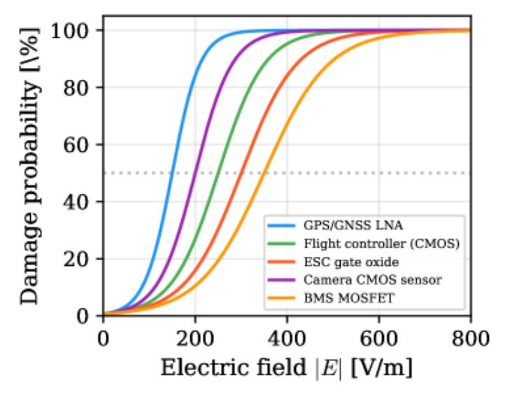
Table 1 summarises the damage model parameters for the five principal drone electronic subsystems, derived from published experimental and simulation studies.

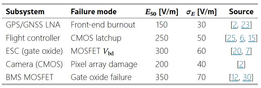
Subsystem	Failure mode	E_50 [V/m]	σ_E [V/m]	Source
GPS/GNSS low-noise amplifier (LNA)	Front-end burnout	150	30	[2, 23]
Flight controller	CMOS latchup	250	50	[25, 6, 15]
ESC (gate oxide)	MOSFET breakdown voltage overload (V_bd)	300	60	[20, 7]
Camera (CMOS)	Pixel array damage	200	40	[2]
BMS (MOSFET)	Gate oxide failure	350	70	[12, 30]

Table 1: Semiconductor damage model parameters for sUAS electronic subsystems. E_50 represents the 50% damage threshold and σ_E represents the transition width.

A drone is considered neutralised if any one of its critical subsystems is damaged, since the loss of either motor control (ESC failure), flight stabilisation (flight controller failure), or navigation (GPS failure) results in an uncontrolled descent. The system-level kill probability is therefore:

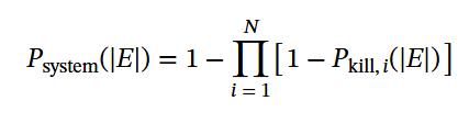
where the product extends over all N vulnerable subsystems.

2.5 Waveguide transmission analysis

The RF power is transported from the magnetron to the feed horn through a WR-340 rectangular waveguide (a=86.36 mm, b=43.18 mm). The cutoff frequency of the dominant TE₁₀ mode is:

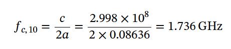
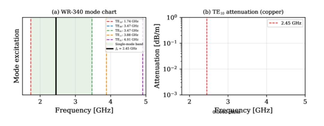
At the operating frequency of 2.45 GHz, only the TE₁₀ mode propagates, since the next mode (TE₂₀) cuts off at 3.471 GHz. The wall-loss attenuation of the TE₁₀ mode in a copper waveguide is [3]:

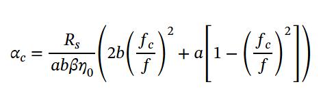
where Rs=πfμ0/σCu is the surface resistance, β is the propagation constant, and σCu=5.8×107 S/m. At 2.45 GHz this yields αc≈0.009 dB/m, confirming negligible loss over a typical 1 m waveguide run.

3. Simulation Framework

The simulation framework is implemented in Python 3.12 using NumPy, SciPy, and Matplotlib. It comprises three tiers: (i) deterministic parametric analysis, (ii) Monte Carlo uncertainty propagation, and (iii) design-space exploration. The complete source code (approximately 400 lines) is provided for full reproducibility.

3.1 Deterministic parametric model

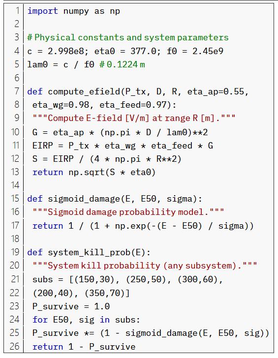
The deterministic model evaluates Eqs. (1)–(7) for specified system parameters. Listing 1 shows the core computation.

3.2 Monte Carlo uncertainty propagation

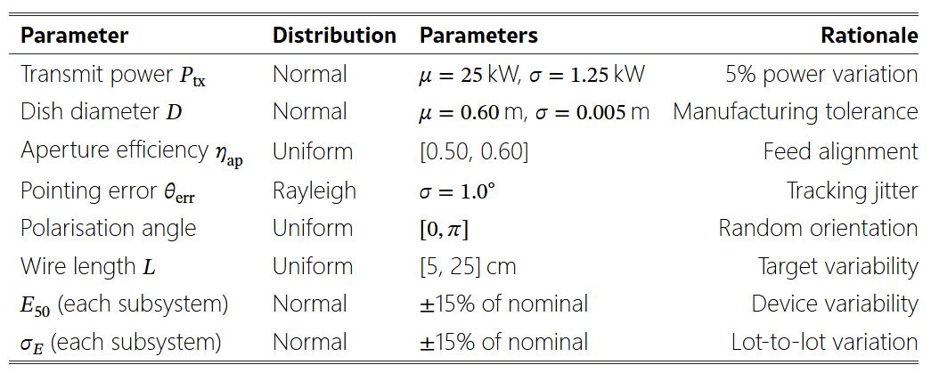
To quantify the effect of parameter uncertainty on system performance, a Monte Carlo simulation with NMC=10,000 independent trials is performed. In each trial, the following parameters are sampled from their respective distributions:

Parameter	Distribution	Distribution parameters	Rationale / physical basis
Transmitter power (P_tx)	Normal	μ = 25 kW, σ = 1.25 kW	5% power fluctuation
Dish diameter (D)	Normal	μ = 0.60 m, σ = 0.005 m	Manufacturing tolerance
Aperture efficiency (η_ap)	Uniform	[0.50, 0.60]	Feed alignment error
Pointing error (θ_err)	Rayleigh	σ = 1.0°	Tracking jitter
Polarisation angle	Uniform	[0, π]	Random attitude orientation
Wire length (L)	Uniform	[5, 25] cm	Target variability (size differences across platforms)
E_50 (each subsystem)	Normal	±15% of nominal	Device-to-device variation
σ_E (each subsystem)	Normal	±15% of nominal	Lot-to-lot variation

Table 2: Monte Carlo parameter distributions. All distributions are truncated to physical limits.

The pointing error is modelled as a Rayleigh-distributed angular offset, producing a Gaussian loss factor Gpointing=exp(−2.76θnorm2) where θnorm=θerr/(θ3dB/2) [3]. The polarisation mismatch efficiency is ηpol=cos2ϕ, bounded below at 0.1 to account for cross-polarised coupling. Listing 2 shows the Monte Carlo core loop.

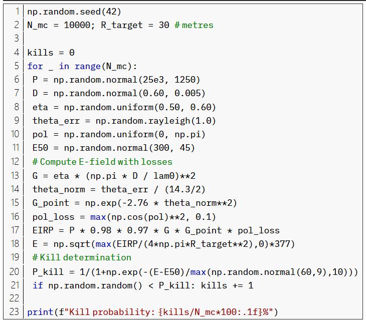
Confidence intervals for the kill probability are computed using the Clopper–Pearson exact binomial method at the 95% level.

4. Results and Discussion

4.1 Electric field distribution

Fig. 2 presents the computed electric field intensity as a function of range for five transmitter power levels, using the baseline 60 cm dish. The field decays as 1/R in accordance with Eq. (2). At the baseline power of 25 kW, the E-field at 20 m is 495 V/m and decreases to 247 V/m at 40 m. The horizontal dashed lines indicate the 50% damage thresholds for CMOS latchup onset (200 V/m) and ESC gate oxide breakdown (300 V/m).

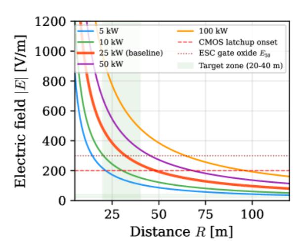
The intersection of the E-field curve with the damage thresholds defines the effective kill range for each subsystem. For 25 kW CW, the E-field exceeds the GPS LNA burnout threshold (150 V/m) out to approximately 65 m, but drops below the ESC gate oxide threshold (300 V/m) at approximately 25 m in CW mode, motivating the use of pulsed operation for extended range.

4.2 CMOS damage probability characterisation

Fig. 3 shows the sigmoid damage probability curves for each drone subsystem as a function of incident electric field. The GPS/GNSS front-end LNA is the most susceptible subsystem (E50=150 V/m), consistent with the low input power tolerance of low-noise amplifiers [2, 37, 33]. The ESC gate oxide represents the primary hard-kill mechanism (E50=300 V/m), requiring higher field strengths but resulting in irreversible motor control loss [20, 7]. The ordering of subsystem susceptibilities (GPS<Camera<FC<ESC<BMS) is consistent with the published hierarchy reported by Bäckström and Lovstrand [2] and the recent HPM-on-UAV experiments of Zhang et al. [40].

4.3 System-level kill probability

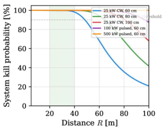
Fig. 4 presents the system-level kill probability (Eq. 7) versus range for five system configurations spanning both CW and pulsed operation with varying dish sizes. At the baseline configuration (25 kW CW, 60 cm dish), the kill probability exceeds 90% at approximately 18 m and falls to approximately 30% at 40 m. Increasing the dish diameter to 100 cm extends the 90% kill range to approximately 26 m owing to the 4.4 dB gain increase. The most dramatic improvement is achieved through pulsed operation: at 500 kW peak power (1% duty cycle, 5 kW average), the 90% kill range extends to approximately 88 m, well beyond the design objective of 40 m.

4.4 Pulsed versus CW operation

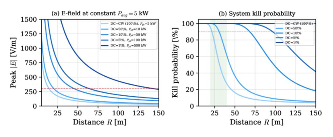
A critical design trade-off is the choice between CW and pulsed operation. Fig. 5 compares both modes at a constant average power budget of 5 kW, demonstrating that reducing the duty cycle increases the peak E-field and therefore extends the effective engagement range. At 1% duty cycle (500 kW peak), the peak E-field at 40 m exceeds 1,100 V/m—well above all damage thresholds. The physical mechanism is twofold: (i) peak voltage-driven breakdown of gate oxides occurs on individual pulses regardless of average power, and (ii) the peak-to-average power ratio directly translates to range extension via the 1/R2 dependence [3, 14, 10].

1. Peak-voltage-driven breakdown: Regardless of average power, the high peak voltage of a single pulse can directly trigger gate-oxide breakdown.

2. Range extension mechanism: The peak-to-average power ratio translates directly into greater effective range through the 1/R^2 energy decay with distance [3, 14, 10].

4.5 Electromagnetic coupling to drone wiring

Fig. 6 shows the induced voltage on drone wiring harnesses as a function of wire length for four incident E-field levels. A pronounced resonance peak occurs near λ0/2=6.12 cm, where the wire acts as a half-wave dipole. At 300 V/m (the baseline E-field at 25 m), the induced voltage on a 6 cm wire reaches approximately 45 V—exceeding the typical MOSFET gate oxide breakdown voltage of 20–40 V [7, 20]. This confirms that unshielded ESC signal wires in the λ/2 range are the most vulnerable coupling path, consistent with the experimental observations of Zhang et al. [40] who reported HPM-induced ESC shutdown as the primary failure mode.

4.6 Monte Carlo uncertainty analysis

Fig. 7 presents the results of the 10,000-trial Monte Carlo simulation. Fig. 7(a) shows the probability distribution of the E-field at R=30 m, which exhibits a roughly normal shape with mean μ=205 V/m and standard deviation σ=80 V/m. The significant spread (coefficient of variation ≈39%) is dominated by the polarisation mismatch and wire orientation uncertainty, demonstrating that deterministic calculations substantially overestimate system performance by ignoring these real-world degradation factors.

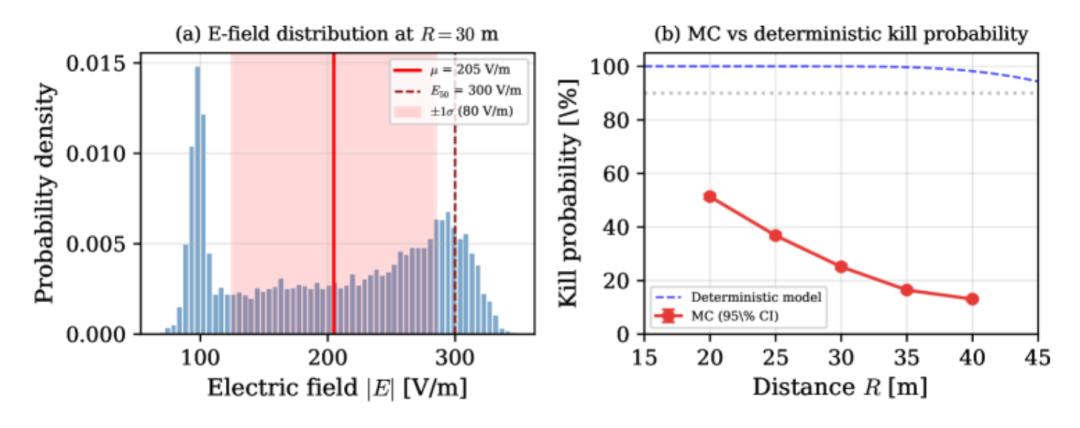
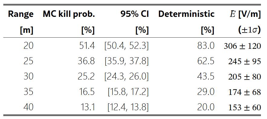
Fig. 7(b) compares the Monte Carlo kill probabilities with 95% confidence intervals against the deterministic model. The Monte Carlo results are systematically lower than the deterministic predictions at all ranges, reflecting the compounding effect of multiple loss mechanisms that are averaged rather than assumed at their best-case values. Table 3 summarises the quantitative results.

Range R [m]	Monte Carlo kill probability [%]	95% CI [%]	Deterministic kill probability [%]	Mean E-field Ē [V/m] (±1 σ)
20	51.4	[50.4, 52.3]	83.0	306 ± 120
25	36.8	[35.9, 37.8]	62.5	245 ± 95
30	25.2	[24.3, 26.0]	43.5	205 ± 80
35	16.5	[15.8, 17.2]	29.0	174 ± 68
40	13.1	[12.4, 13.8]	20.0	153 ± 60

The Monte Carlo analysis reveals that the deterministic model overestimates the kill probability by a factor of approximately 1.5–1.6× across the engagement zone. This discrepancy highlights the necessity of stochastic analysis for realistic performance prediction, a finding consistent with the susceptibility variability reported in [2, 23, 8].

4.7 Parametric design space

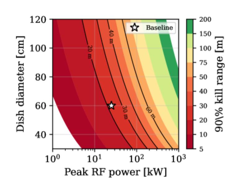
Fig. 8 presents a contour map of the 90% kill range as a function of peak RF power and dish diameter, enabling rapid system-level design trade studies. The baseline design point (25 kW, 60 cm) is marked. The contours reveal that the kill range scales approximately as R90∝P⋅D2, as expected from the 1/R2 power density dependence combined with the D2 antenna gain scaling. This parametric map provides a practical tool for system designers to evaluate the power–aperture trade space against specific operational requirements.

4.8 Antenna design analysis

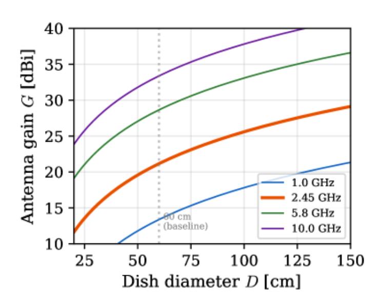
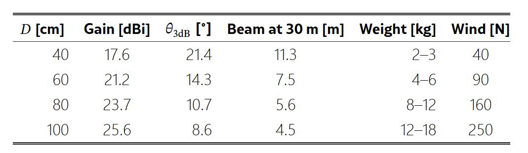
Fig. 9 presents the antenna gain versus dish diameter at four frequencies. At 2.45 GHz, a 60 cm dish yields 21.2 dBi gain, while a 100 cm dish provides 25.6 dBi. The gain–size trade-off is important for mobile systems where weight, wind load, and agility constraints limit the maximum dish diameter [3]. Table 4 summarises the trade analysis.

4.9 Beam footprint analysis

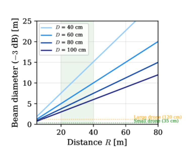
Fig. 10 shows the −3 dB beam diameter as a function of range for four dish sizes. At 30 m with the 60 cm baseline dish, the beam footprint is 7.5 m—approximately 15× the physical size of a typical sUAS. This generous beam size relaxes tracking accuracy requirements and provides inherent robustness against pointing jitter, a significant advantage over laser-based systems that require sub-milliradian precision [1, 17].

4.10 Waveguide mode and attenuation analysis

Fig. 11 presents the WR-340 waveguide analysis. Fig. 11(a) shows the mode chart with cutoff frequencies for the five lowest-order modes. At 2.45 GHz, only the TE₁₀ mode propagates, confirming single-mode operation. The single-mode bandwidth extends from 1.736 GHz to 3.471 GHz, providing substantial margin for magnetron frequency drift (typically ±10 MHz). Fig. 11(b) shows the TE₁₀ attenuation in copper, which at 2.45 GHz is only 0.009 dB/m, resulting in negligible loss over the typical 1 m waveguide run.

4.11 Thermal management

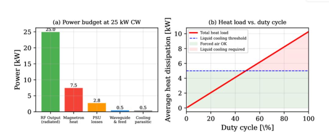
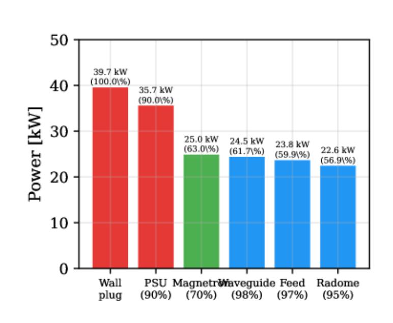
Fig. 12 presents the thermal analysis. At 25 kW CW operation with 70% magnetron efficiency, the system dissipates 7.5 kW in the magnetron body and an additional 4.0 kW in the PSU (90% efficiency), for a total thermal load of approximately 12 kW. Fig. 12(a) shows the power budget breakdown, and Fig. 12(b) illustrates the average heat load as a function of duty cycle. Liquid cooling is required above approximately 40% duty cycle (5 kW heat threshold), while pulsed operation at ≤5% duty cycle permits forced-air cooling, significantly simplifying the system for mobile deployment.

• Above approximately 40% duty cycle (corresponding to a 5 kW heat dissipation threshold), the system requires liquid cooling;

• while pulsed operation at ≤5% duty cycle permits forced-air cooling, greatly simplifying the thermal design and favouring mobile deployment.

4.12 System efficiency chain

Fig. 13 shows the power flow from wall plug to radiated RF, illustrating the cumulative effect of losses at each stage. The overall wall-plug-to-radiated efficiency is approximately 58%, consistent with the high DC-to-RF efficiency of cavity magnetrons [29, 34, 19, 13]. The magnetron is the dominant loss mechanism (30% of input power converted to heat), followed by the PSU (10% losses).

5. Discussion

The simulation framework presented in this paper provides several insights for HPM C-UAS system design that merit discussion.

First, the Monte Carlo analysis demonstrates that deterministic link-budget calculations overestimate kill probability by approximately 60% (Table 3). This overestimation arises primarily from the polarisation mismatch and wire orientation randomness, which introduce a multiplicative loss factor that is unity only in the best case and averages to ⟨cos2ϕ⟩=0.5 over a uniformly distributed orientation. This finding underscores the importance of stochastic analysis for realistic C-UAS performance prediction and has implications for system specification: to guarantee 90% kill probability at a given range, the system must be designed with 5–8 dB margin above the deterministic threshold.

Second, the pulsed operating mode provides the most effective path to extending engagement range within practical size, weight, and power (SWaP) constraints. At 1% duty cycle, the 90% kill range increases by approximately 4.7× relative to CW operation at the same average power. This advantage is further amplified by the voltage-driven (rather than thermal) damage mechanism in pulsed mode, which requires only a few microsecond-duration pulses rather than seconds of continuous illumination [14, 10].

Third, the resonance-enhanced coupling model (Eq. 5) identifies drone wiring harnesses in the 5–8 cm range as the critical vulnerability path at 2.45 GHz. This finding is consistent with the recent experimental results of Zhang et al. [40], who reported that HPM irradiation caused GPS interference, datalink interruption, and ESC shutdown in consumer UAVs, with internal cable coupling identified as the primary energy entry mechanism.

A comparison with fielded systems provides context for the simulation results. The Epirus Leonidas system uses solid-state GaN amplifier arrays rather than magnetrons, achieving software-defined beam control and demonstrated 100% effectiveness against swarms of up to 49 drones. While the exact Leonidas operating parameters are not publicly disclosed, the system reportedly operates at power levels consistent with the pulsed configurations analysed in this study [21]. The Raytheon Phaser, which uses a traditional HPM source architecture more similar to the system modelled here, has also demonstrated operational effectiveness in field trials. The framework developed in this paper enables parametric comparison of such architectures within a unified analytical framework.

Several limitations should be acknowledged. The damage probability model (Eq. 6) assumes far-field plane-wave illumination and does not capture near-field effects that become significant below approximately 2D2/λ=5.9 m for the 60 cm dish. The sigmoid parameters in Table 1 are derived from published literature spanning different experimental setups and device technologies; dedicated susceptibility testing of specific sUAS models would refine these values. The electromagnetic coupling model treats the wiring as an isolated short dipole and does not account for the complex electromagnetic environment inside a drone airframe, including mutual coupling between conductors and cavity resonances within the enclosure [9]. Finally, atmospheric effects (humidity, rain) are neglected, which is reasonable at 2.45 GHz where atmospheric attenuation is <0.01 dB/km in clear air but may become significant in heavy precipitation.

6. Conclusions

This paper has presented a multi-physics simulation framework for the design and performance evaluation of high-power microwave counter-UAS systems. The framework integrates RF propagation, antenna pattern analysis, electromagnetic coupling to unshielded drone electronics, and a probabilistic semiconductor damage model into a unified computational tool. The principal findings are as follows.

1. For a baseline 25 kW CW system with a 60 cm dish, the Monte Carlo simulation yields a kill probability of 51.4% (95% CI: [50.4, 52.3]%) at 20 m and 13.1% (95% CI: [12.4, 13.8]%) at 40 m, with the deterministic model overestimating performance by approximately 1.6×.

2. Pulsed operation at 500 kW peak power (1% duty cycle) extends the 90% kill range from approximately 18 m to 88 m while maintaining a manageable average power of 5 kW, which permits forced-air rather than liquid cooling.

3. The resonance-enhanced electromagnetic coupling model identifies drone wiring harnesses in the 5–8 cm range (near λ0/2 at 2.45 GHz) as the critical vulnerability path, with induced voltages exceeding the 20–40 V MOSFET gate oxide breakdown threshold at field strengths above 200 V/m.

4. The parametric design map reveals that the 90% kill range scales as P⋅D2, providing a practical tool for power–aperture trade studies.

5. ICNIRP-compliant safety exclusion zones of 72 m (occupational) and 161 m (general public) are required at 25 kW CW in the main beam, decreasing proportionally in pulsed mode.

Future work will extend the framework to include full-wave electromagnetic simulation of drone airframes using finite-difference time-domain (FDTD) methods, validation against controlled HPM exposure experiments on representative sUAS platforms, and integration of tracking system dynamics into the engagement probability model.

Acknowledgements

The authors state that the style and English of this work has been polished using AI tools provided by QuillBot. There is no funding associated with this work.

If you have any questions about this topic, feel free to contact us at [email protected].

Have questions about this article? Feel free to contact us at [email protected] — we’re happy to help!