
Key Takeaways
- A fixed-wing UAV flying a tracking task must satisfy convergence-time and steady-state error requirements while staying clear of static and dynamic obstacles.
- Avoidance manoeuvres push the aircraft off its reference path, so the two requirements genuinely conflict.
- The 2026 paper in Aerospace Science and Technology combines prescribed performance control, a predefined-time disturbance observer and a control barrier function inside one quadratic program.
- The observer converges within a preset 2 seconds; per-axis tracking error settles inside 0.1 m within 10 seconds.
- Results are numerical only — the authors report no hardware flight test, and QP feasibility under input saturation remains open.
Fixed-wing UAV trajectory tracking under unknown disturbances and obstacles has to satisfy two things at once: convergence time and steady-state error, and a safe separation from static and dynamic obstacles. As of 2026 the practical difficulty is that the avoidance manoeuvre itself enlarges tracking error, which can break the performance envelope the controller was designed around.
The paper reviewed here, Collision-Free Robust Trajectory Tracking Control for Fixed-Wing UAV with Flexible Performance Constraints, brings prescribed performance control, a predefined-time disturbance observer and a control barrier function into a quadratic programming framework. When safety and performance collide, it corrects the nominal control input and adaptively relaxes the performance boundary, reconciling avoidance with tracking. The work is validated by theory and numerical simulation only; the “flexible” in the title refers to that adaptive relaxation of the tracking error boundary.
Three Reasons the Problem Is Hard
Tracking accuracy and avoidance safety can conflict
Prescribed performance control bounds the tracking error within a predefined envelope, which is how overshoot, convergence time and steady-state accuracy get specified. During avoidance the controller must push the aircraft off the reference trajectory, and tracking error grows accordingly. If the performance requirement is held fixed, the actual error can cross the boundary and trigger the singularity that prescribed performance control is prone to.
Unknown disturbances undermine model-based safety constraints
A control barrier function builds its safety constraint from the system model, so unknown disturbances can drive the state outside the safe set. A robust control barrier function that assumes a worst-case disturbance bound does guarantee safety, but it can make the admissible safe input set far too conservative. Existing observer-plus-CBF schemes also carry either an estimation-error ceiling or an asymptotic-convergence restriction.
The performance function must handle both initial error and quantitative targets
When the system restarts or the desired state changes, some existing performance functions must be redesigned and their initial conditions re-checked. An initial boundary that is too wide degrades transient performance, while methods tied to the initial error struggle to prescribe convergence time exactly. The authors therefore design a polynomial performance function parameterised by the initial error.
The Architecture: Performance as the Baseline, Safety as the Correction
The framework runs in three layers. A prescribed-performance controller generates a nominal input. A control barrier function combined with the predefined-time disturbance observer builds the avoidance constraint. A quadratic program then makes the smallest possible correction to the nominal input. The input error between the safe control and the nominal control is fed back to an auxiliary system, which drives the boundary adjustment.
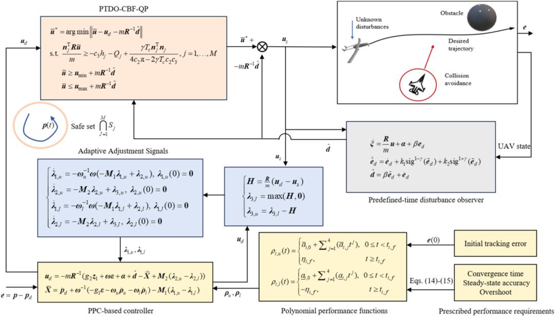
- Performance control: a polynomial performance function prescribes how the tracking error may evolve, and an error transformation plus controller design keeps the constraint satisfied.
- Disturbance estimation and safety correction: the predefined-time observer estimates the lumped disturbance, the control barrier function converts the safety-distance requirement into a constraint on the control input, and the quadratic program returns a safe input that satisfies it.
- Boundary feedback adjustment: when the safety correction degrades tracking performance, a non-negative adaptive signal relaxes the error boundary. Once the safe input returns to the nominal one, the signal decays and the boundary recovers.
The Fixed-Wing Model
The model takes thrust, lift and roll angle as control inputs, written in a compact translational form over position and velocity. The analysis that follows is built on it, and the paper assumes the desired trajectory is twice continuously differentiable and bounded.
For simulation convenience the paper defines an indirect control input u = [T, Lcosφ, Lsinφ]T, where T, L and φ are thrust, lift and roll angle. The input bounds quoted later apply to that vector, with every component in newtons.
Prescribing the Error Boundary with a Polynomial
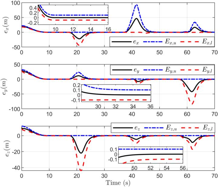
For each axis the authors design separate upper and lower performance boundaries. Before the convergence time the boundary follows a quartic polynomial; after it, the boundary holds at the specified steady-state error tolerance. The initial error enters the design explicitly, so it always starts inside the boundary. The polynomial coefficients are fixed by the initial value, the terminal value and the corresponding derivative conditions.
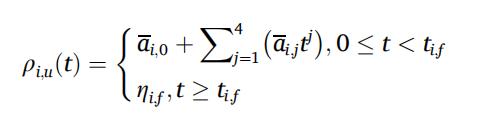
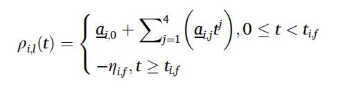
Here ti,f is the prescribed convergence time for axis i and ηi,f is the steady-state error tolerance. The upper and lower coefficient sets are each solved from the initial boundary value, terminal boundary value and derivative conditions.
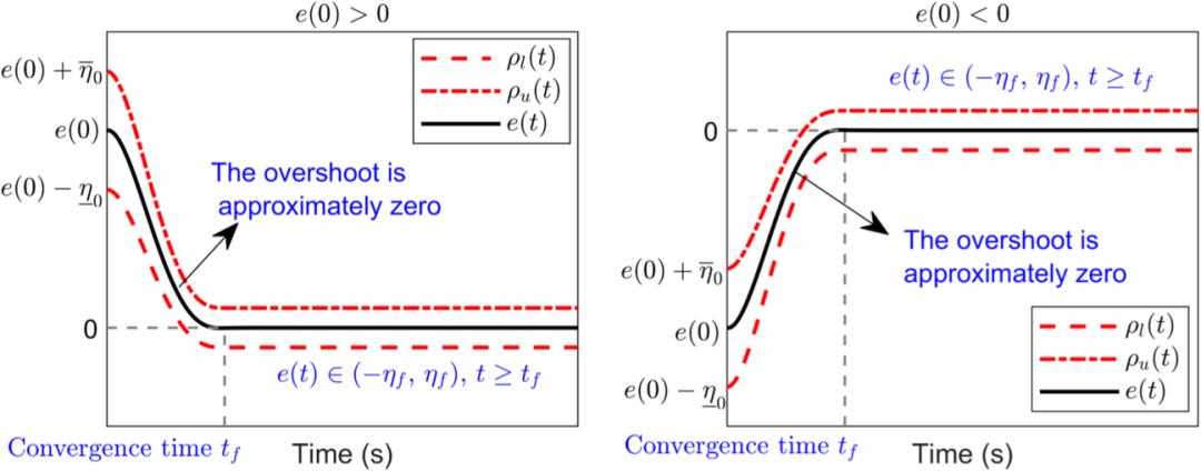
The figure shows the boundary and the error evolution for both positive and negative initial error. Parameter choice sets the convergence time and steady-state tolerance, and the envelope can be tightened to reduce overshoot.
Relaxing the Boundary Without Relaxing Safety
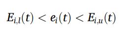
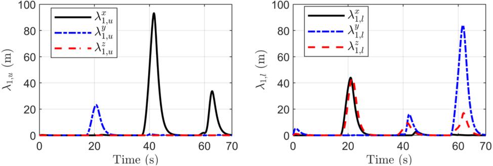
The adjusted upper boundary becomes Ei,u(t) = ρi,u(t) + λ1,ui(t) and the lower boundary Ei,l(t) = ρi,l(t) − λ1,li(t). Adding a non-negative adjustment to the upper bound and subtracting one from the lower keeps the tracking error evolving inside the adjusted envelope. What relaxes is the tracking performance boundary; the obstacle safety distance never changes.
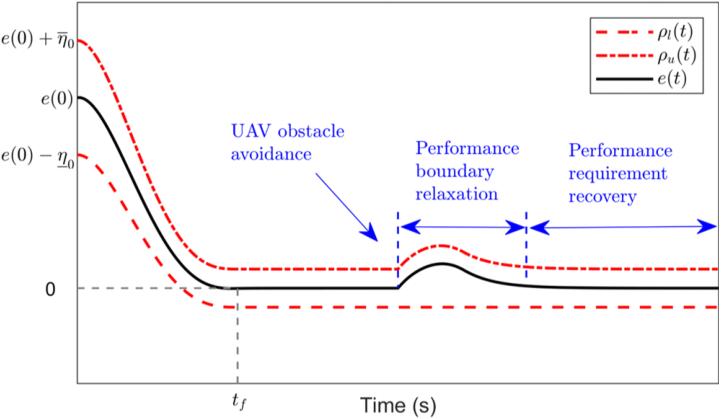
The auxiliary system is driven by the difference between the nominal and the safe control input. The authors use positive system theory to guarantee the adjustment signal stays non-negative, and to quantify how much performance the safety constraint costs. With input saturation considered, the same signals quantify the performance cost of saturation. When the safe input equals the nominal one, the auxiliary system’s driving term is zero, the adjustment signal decays exponentially under the damping term, and the boundary recovers.
Estimating the Lumped Disturbance in Predefined Time
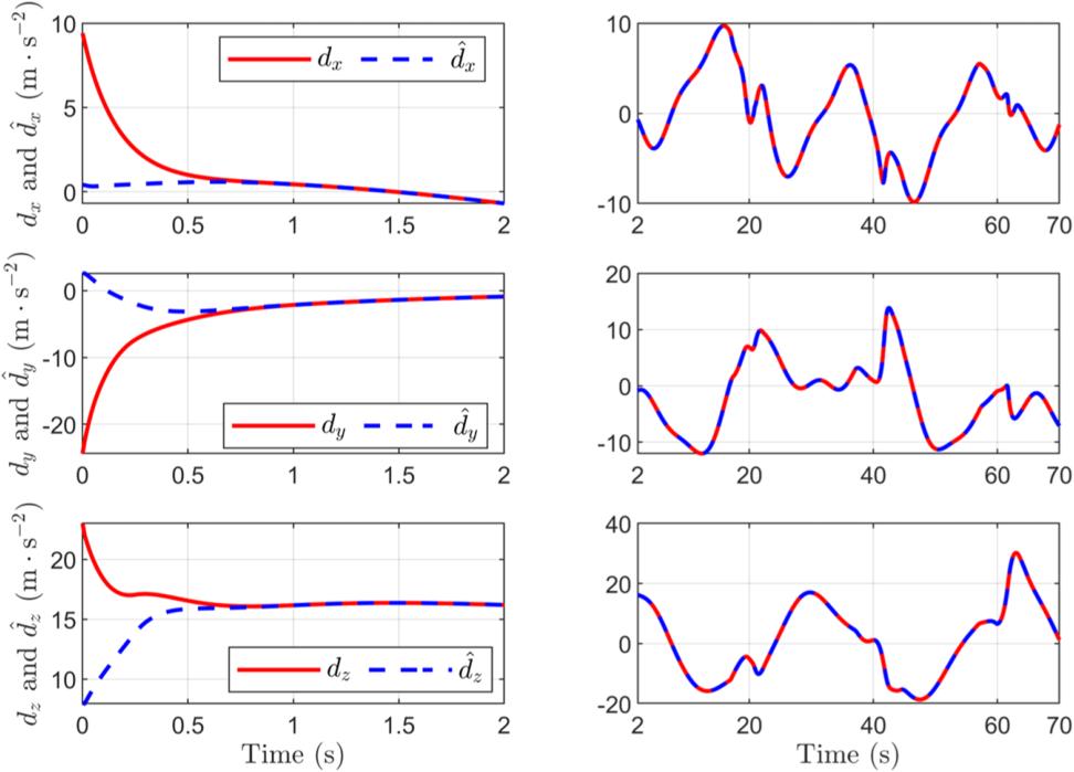
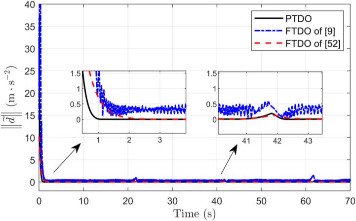
The predefined-time disturbance observer estimates the lumped disturbance in the model, analysed with a Lyapunov function, and the paper proves that the estimation error converges to zero within the preset time Tc. The convergence proof goes further: for all t ≥ Tc, the disturbance estimation error is zero.
Within the performance loop, the boundary-constrained error is transformed into an unconstrained one, a virtual velocity command is constructed, and a prescribed-performance tracking controller is designed that includes disturbance-estimate compensation. Under the stated trajectory assumptions and the designed performance function, auxiliary system, observer and controller, the closed loop is shown to be uniformly bounded, with tracking error satisfying the adjusted performance boundary.

Here ud is the nominal control input, z1 = v − vd is the intermediate velocity error, ε is the transformed error and d̂ is the lumped disturbance estimate. The gains, matrices and auxiliary terms follow from the error transformation, the auxiliary system and the controller design.
Turning Safety Distance into a Constraint
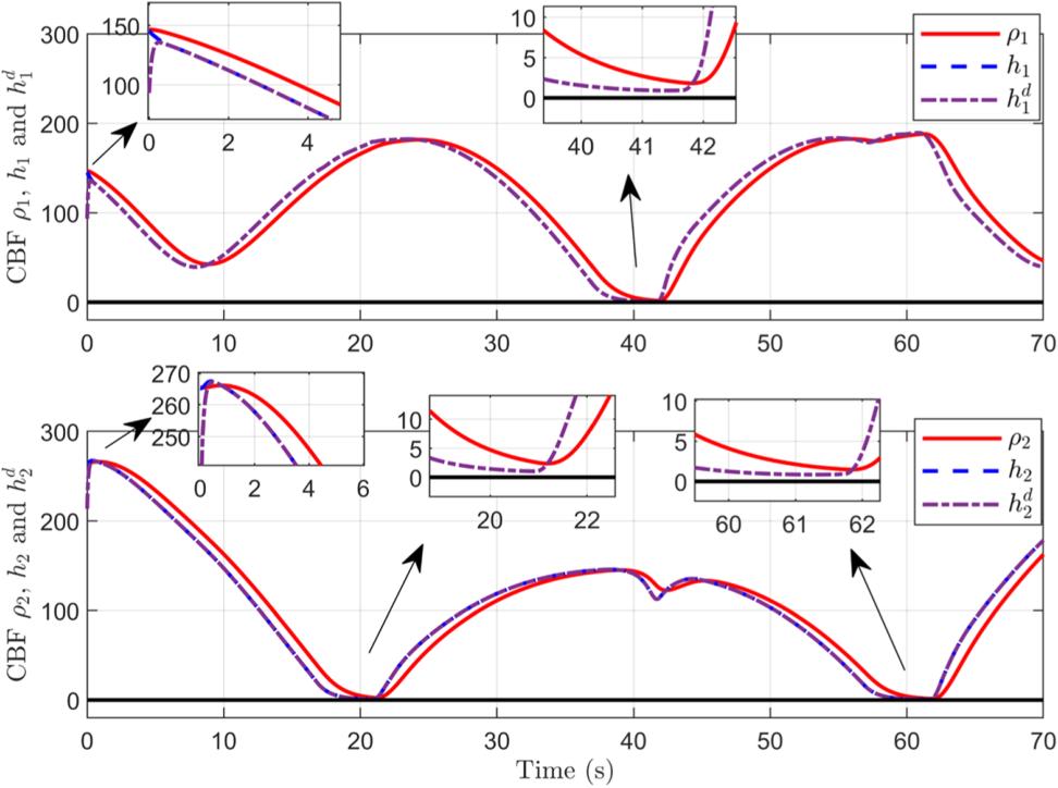
The authors define a distance function ρj(t) as the centre distance between the UAV and the obstacle, minus the obstacle radius rj and an additional safety margin rs. So ρj ≥ 0 means the prescribed avoidance distance is satisfied.

Here δj(t) = p(t) − pj(t) is the relative position vector between the UAV and obstacle j.
Because the distance function has relative degree 2 with respect to the control input, the authors introduce a high-order control barrier function and correct the barrier term with the Lyapunov function of the disturbance estimation error, producing a robust safety constraint built on the predefined-time observer. As the estimation error converges within the preset time, the influence of that error on the barrier correction disappears.
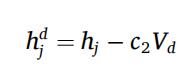
Here hj = ρ̇j + c1ρj, Vd is the Lyapunov function of the disturbance estimation error, c1 and c2 are positive constants, and hjd is the corrected barrier term.
The Quadratic Program
Safety enters as a hard constraint, and the objective is to stay as close as possible to the nominal control input. Performance requirements are reconciled through minimal input correction and adaptive boundary relaxation.
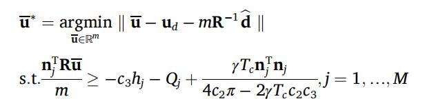
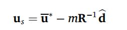
Here ū is the optimisation variable, ū* the optimum, and the final safe control input is the optimum minus the disturbance compensation term. m is the UAV mass, R the input transformation matrix of the compact translational model and d̂ the lumped disturbance estimate. nj = δj/‖δj‖ is the unit vector along the relative position, and Qj collects the model terms, the obstacle acceleration and the relative position and velocity.
The safety proof requires the initial distance for every obstacle to satisfy ρj(0) ≥ 0 and the corrected barrier initial condition hjd(0) > 0. Parameters must also satisfy c3 > 0 and 2π − γTcc3 > 0, and the conclusions hold subject to the model assumptions and to the optimisation problem being feasible.
When the nominal input already satisfies the avoidance constraint, the program keeps it; otherwise it applies the smallest correction. If input saturation constraints are added, keeping the nominal input also requires it to lie inside the input bounds. The paper states explicitly that QP feasibility under input saturation is still an open problem.
Simulation Setup
All validation is numerical. The simulation first examines tracking and avoidance from different initial positions, then uses case 3 to show error, performance boundaries, disturbance estimates, safety variables and control inputs, and compares against a fixed-time disturbance observer and other CBF-based controllers.
| Parameter | Value |
|---|---|
| UAV mass | 5 kg |
| Obstacles | One static and one dynamic sphere, radius 10 m each |
| Additional safety margin | 10 m, so required centre distance ≥ 20 m |
| Desired trajectory | pd(t) = [100cos(0.2t), 100sin(0.2t), 2t]T m |
| Prescribed convergence time | 10 s on each axis |
| Steady-state error tolerance | 0.1 m on each axis |
| Observer preset time | 2 s, with γ = 0.3 |
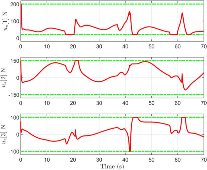
| Input upper bound | umax = [200, 150, 100]T N |
| Input lower bound | umin = [20, −150, −100]T N |
| Initial positions | [50, 10, 0]T, [30, −20, −15]T, [120, 30, 10]T m |

Time-varying disturbances are injected into the state equations for position, airspeed, flight path angle and heading angle.
Results
In all three cases the UAV avoids both the static and the dynamic obstacle and completes the reference tracking. Because the performance function accounts for the initial tracking error explicitly, changing the initial position requires no manual retuning of its design parameters.
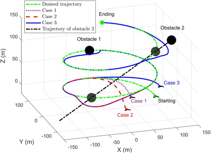
In case 3, with no avoidance needed and the boundary untouched, each axis error enters the ±0.1 m tolerance within the specified 10 seconds. During avoidance the adaptive signal relaxes the performance boundary; after the manoeuvre it converges back to zero and the original requirement is restored. The steady-state tolerance in this simulation is specified per axis, 0.1 m in each case.
The predefined-time observer estimates the lumped disturbance accurately within the specified 2 seconds. Compared under identical initial conditions and disturbances against the fixed-time observers of references [9] and [52], it converges faster and estimates more accurately, and its convergence time can be specified in advance.
In case 3 the distance functions for both obstacles stay non-negative throughout, so the simulated trajectory meets the safety distance requirement. After the preset time the corrected barrier term coincides with the original one, and the control input stays within its bounds.
Comparison with CBF and Robust CBF Controllers
The comparison controllers use the control barrier function of reference [32] and the robust control barrier function of reference [44], both built through quadratic programming with input constraints considered, under the same settings as case 3.
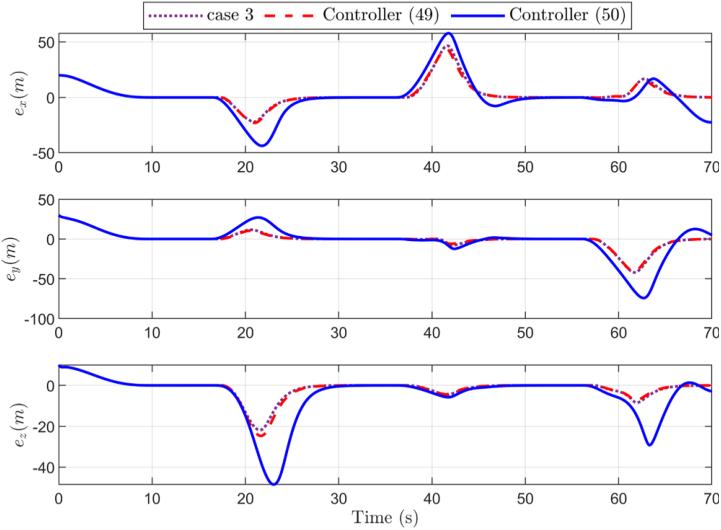
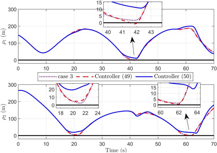
- Plain CBF controller: ρ1 goes negative at approximately 41.5 s, so the safety margin is violated.
- Robust CBF controller: safety is maintained, but designing against a disturbance upper bound pushes the avoidance distance well beyond the required margin and costs substantial tracking error.
- Proposed method: the observer-based CBF keeps the avoidance safe while preserving tracking performance better than the robust CBF scheme it is compared against.
Conclusions and Open Problems
The paper proposes a safety control strategy for fixed-wing UAV tracking under unknown disturbances and obstacles with flexible performance constraints: prescribed performance control sets the performance baseline, the predefined-time disturbance observer estimates the lumped disturbance, the control barrier function and quadratic program apply the safety correction, and a non-negative adaptive signal reconciles the performance cost of avoidance. Theory and simulation show that, under the stated conditions, the method satisfies both avoidance safety and reference tracking.
The authors also state two limitations: input saturation can make the quadratic program infeasible, and the work is validated by numerical simulation only. Future work will target QP feasibility under input constraints and hardware validation of the proposed scheme.
Have questions about this article? Feel free to contact us at [email protected] — we’re happy to help!
Frequently Asked Questions
Why can obstacle avoidance break a fixed-wing tracking controller?
Because avoidance requires deviating from the reference path, which enlarges tracking error. If the prescribed performance boundary is fixed, the error can cross it and trigger the singularity inherent to prescribed performance control.
What does “flexible performance constraints” mean in this paper?
The tracking error boundary relaxes adaptively during an avoidance manoeuvre and recovers afterwards. The obstacle safety distance is never relaxed — only the tracking performance envelope moves.
How fast does the disturbance observer converge?
Within a preset 2 seconds in the simulation, with γ = 0.3. Unlike a fixed-time observer, the convergence time is specified by the designer rather than emerging from the gains.
Was this validated on a real fixed-wing aircraft?
No. All results are numerical simulation. The authors list hardware validation as future work, alongside resolving quadratic program feasibility under input saturation.
How much better is it than a robust control barrier function?
The robust CBF stays safe but is conservative: designing against a worst-case disturbance bound makes the aircraft avoid well beyond the required 20 m centre distance, which shows up as larger tracking error. The proposed observer-based CBF holds the same safety while keeping error closer to the reference.
About Aomway
Aomway has been developing and manufacturing video transmission and UAV radio hardware for over 15 years, producing equipment for any frequency band from 1 GHz to 9 GHz at power levels from 3W to 15W. We build high-power FPV video transmitters, directional and circularly polarised antennas, digital links, fiber-optic tether systems and detection hardware for pilots, integrators and commercial operators worldwide.