
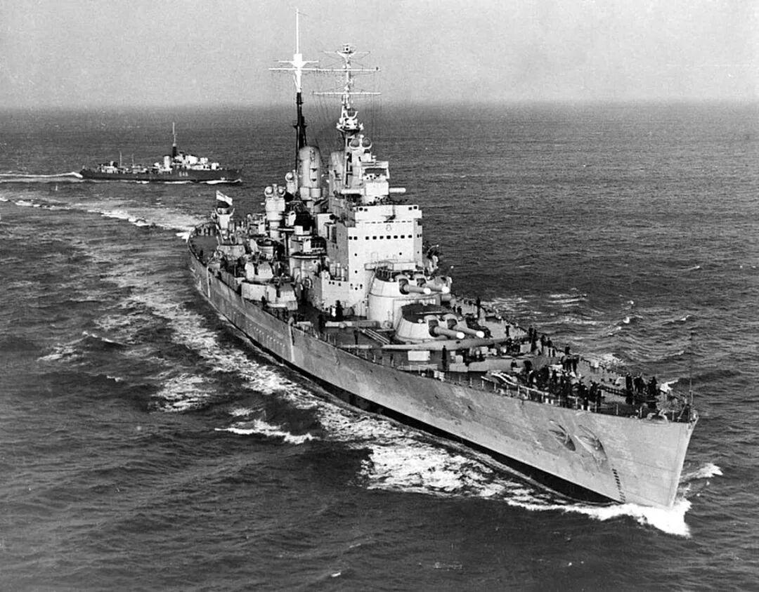
Key Takeaways
- The heavy anti-aircraft fire-control computer aboard HMS Vanguard was the American MK1A, not a British design.
- It fits target course, speed and range rate automatically, with no manual entry of the target’s motion.
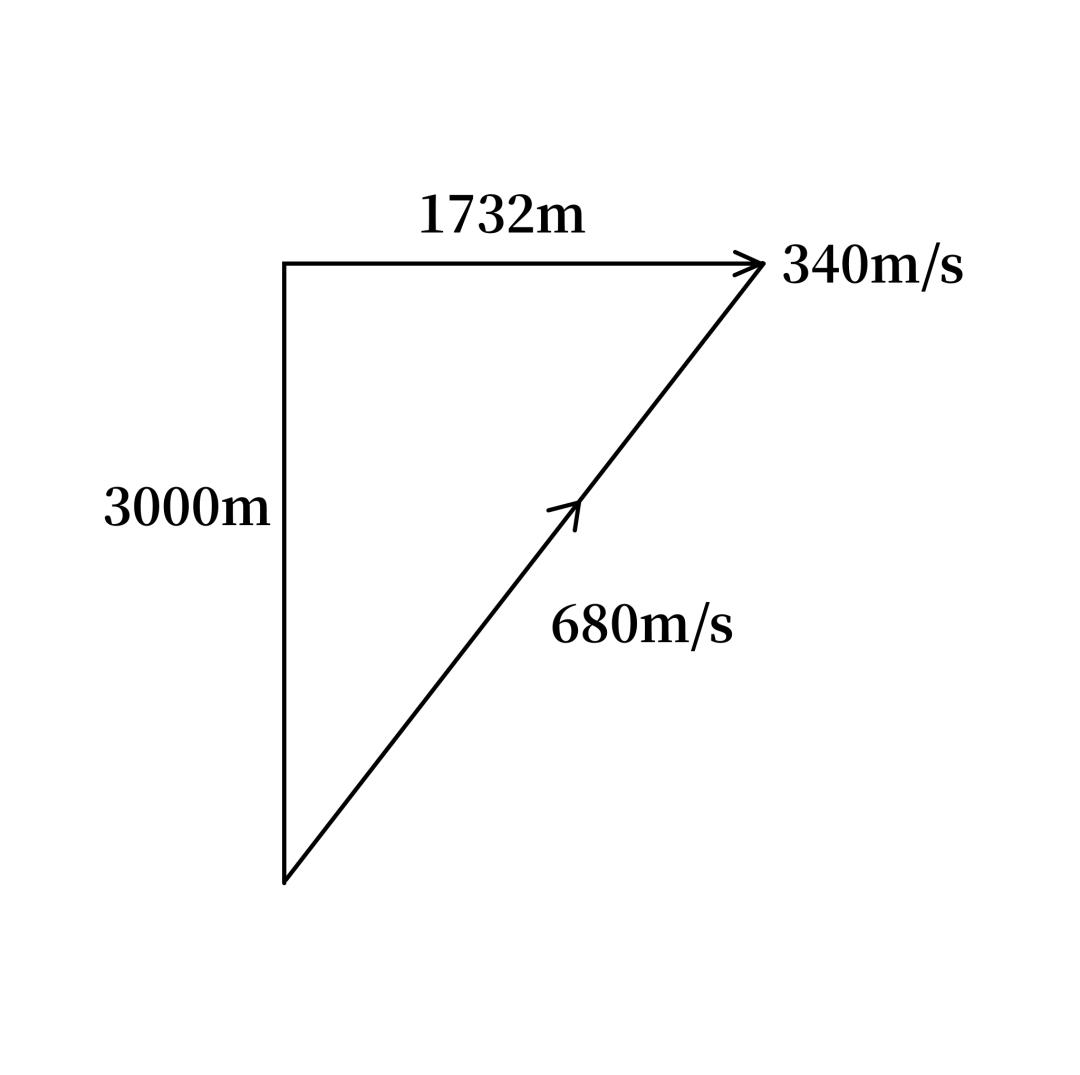
- A 340 m/s crossing target at 3,000 m against a 680 m/s shell yields a 5.1 s time of flight and a 1,732 m intercept offset.
- Ten seconds of steady tracking with the 2-second time-constant gear cuts motion-parameter error to roughly 0.675% of its initial value.
- Every operation is mechanical: ball-disc integrators, wheel-ball component integrators, differentials and follow-up motors.
The MK1A fire-control computer solved a problem most fire-control systems of its generation simply handed to a human: it worked out how the target was moving without being told. As of 2026 it remains the clearest mechanical example of automatic target-motion fitting ever fielded at sea, and the gearing that does the work is worth understanding in detail.
Why the MK1A Had to Solve for Target Motion Itself
For most weapons, computing a fire-control solution means finding the aim direction that will put a projectile on the target. That requires knowing the target’s motion first, because only then can the computer find the future point where projectile and target meet.
Take a concrete case. A target crosses from left to right at 340 m/s perpendicular to the gun’s line of sight. Range is 3,000 m and the shell’s average velocity is 680 m/s. The meeting point satisfies:
3000² + (340t)² = (680t)²
which reduces to 346800t² = 9000000, giving t ≈ 5.1 s. The intercept point sits about 1,732 m to the right of the target’s present position.
The difficulty is obvious: a target does not announce its course and speed. In this mode of fire control the computer must derive the target’s motion state from observation. The MK1A does exactly that on its own.
The Vector Decomposition: Bc, Ec and dR
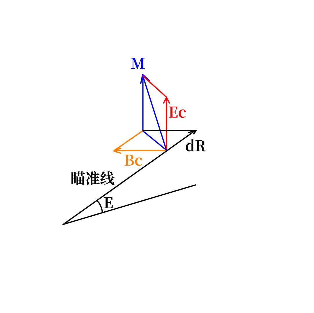
Start with a simple vector-composition problem. Suppose the computer has been set with a target motion vector M. Resolve that vector along three mutually perpendicular directions.
The first component lies in the horizontal plane, perpendicular to the line of sight. It changes the target’s relative bearing, so it is called bearing linear velocity Bc (strictly RdBs), positive to the right. The second lies in the vertical plane, perpendicular to the line of sight, changes the target’s relative elevation, and is called elevation linear velocity Ec (strictly RdE), positive upward. The third runs along the line of sight and changes range, so it is the rate of range change dR, positive opening.
Compose the three and you recover the target’s motion vector:
Bc + Ec + dR = M
But the MK37 director disagrees. To a director that is steadily tracking, the bearing rate is not Bc but Bc′, the elevation rate is not Ec but Ec′, and the range rate is a new value dR′. Compose those and you get the vector the director actually implies:
Bc′ + Ec′ + dR′ = M′
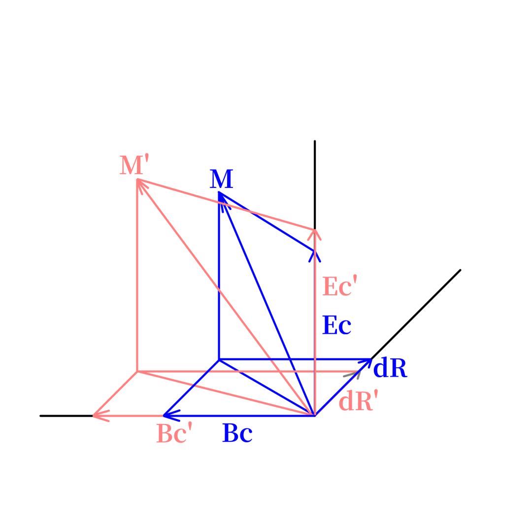
Because Bc′, Ec′ and dR′ differ from Bc, Ec and dR, there must be deviations between them:
Bc′ − Bc = jBc
Ec′ − Ec = jEc
dR′ − dR = jdR
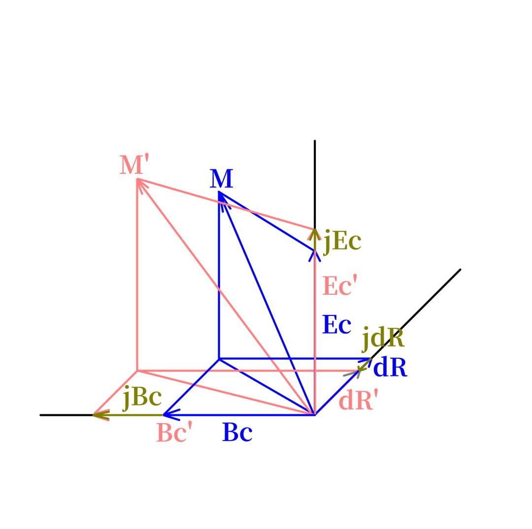
Compose the three deviations and you obtain the gap between M′ and M:
jM = jBc + jEc + jdR
And M′ = M + jM. In other words, if jBc, jEc and jdR can be measured accurately, the target’s motion state can be fitted directly. The only question is how.
Measuring the Deviation: Differentials and Follow-Up Motors
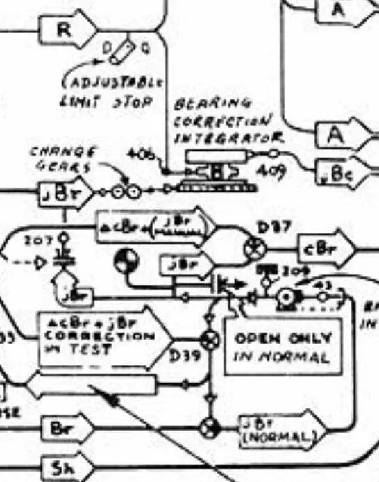
Put the MK1A’s selector to NORMAL and follow the bearing channel.
The MK1A, built by Ford Instrument Company, carries the signature ball-disc integrator. From the target motion state it currently holds, the computer outputs a bearing linear velocity Bc (RdBs). That value sets the position of a friction-ball pair inside a ball-disc integrator. As long as the integrator’s drive disc is turning, the friction balls roll — including at zero speed — and the rolling is taken off through the output shaft on top, rotating the computer’s relative-bearing-rate dial and continuously predicting the current relative target bearing cBr.
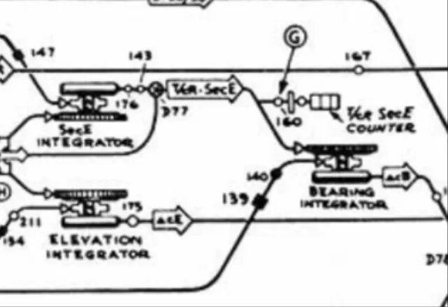
Something else is busy at the same time. The MK37 director, which supplies the MK1A with the observed target position, keeps tracking and continuously sends down its line of sight. That gives the actual relative bearing Br. Because the target keeps moving, both Br and cBr keep changing, and their rates of change are RBr and RcBr — the actual and predicted relative bearing rates.
Subtract one from the other and you get jBr. That is precisely what the MK1A does: a differential D39 in the bearing channel takes cBr on one input shaft and Br on the other. When the two shafts turn at different speeds, the differential’s output shaft turns, and its speed represents jBr.
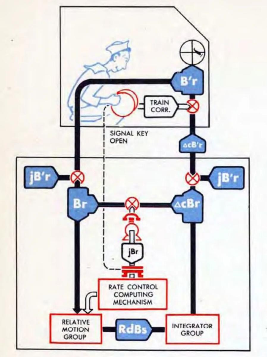
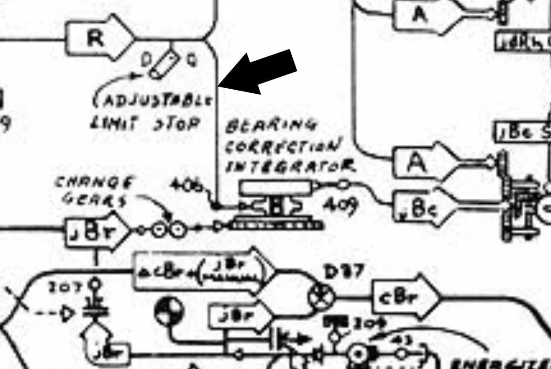
In practice the MK1A is a little more elaborate. The differential’s output shaft drives a contact switch. The moment the switch is displaced, a follow-up motor is energised and turns a follow-up shaft. That motor’s signal has two destinations: one supplies power to a bearing correction integrator with a 3-inch drive disc, and the other is fed back through a second differential where it is added to cBr.
As the follow-up motor starts, the follow-up shaft speeds up, so the cBr shaft entering D39 also speeds up and overtakes Br. Because the two input speeds have now swapped, D39’s output shaft immediately reverses until the contact switch recentres and the motor is cut off. The instant the motor is cut off, the cBr shaft loses its assist and slows down until it falls below Br, the switch is displaced again, and the motor restarts. This pulsing speed regulation holds the motor’s speed very close to jBr.
Why jBr Passes Through an Integrator
Two reasons.
First, jBr is a difference of angular rates, but what is needed to fit the target’s motion is not an angular-rate difference — it is a linear-velocity difference jBc. The angular difference must be multiplied by the current range R, since v = ωR. An integrator performs that multiplication.
Look closely at the 3-inch integrator. Its friction-ball pair is positioned by range R, so the distance from the ball pair to the disc centre can be written kR, where k is a constant of proportionality. When the drive disc turns at jBr, the linear velocity at the ball pair’s position is k × jBr × R — a quantity carrying the bearing linear-velocity difference. The closer the target, the nearer the ball pair sits to the centre, the lower the disc’s linear velocity under it, the slower the balls roll, and the smaller the output jBc. The farther the target, the farther out the ball pair sits, and the larger the output jBc.
The second reason is less widely known: an integrator also filters.
Suppose the relative-bearing-rate difference is 0.01 rad/s (about 0.573°/s) and range is 10,000 m. The bearing linear-velocity deviation works out to 100 m/s. Run the integrator for 10 seconds and the accumulated bearing displacement error is roughly 100 × 10 = 1,000 m.
That is the ideal case. Now inject a jump: for 0.2 s the incoming jBr rises to 0.04 rad/s. During those 0.2 s the integrator outputs 0.04 × 10,000 × 0.2 = 80 m of bearing displacement. Over the remaining 9.8 s it outputs 0.01 × 10,000 × 9.8 = 980 m. The total is 980 + 80 = 1,060 m. Divide by the 10-second integration time and the average bearing linear-velocity deviation is only 106 m/s — just 6% above the original 100 m/s, even though the transient was four times larger. A violent oscillation has been smoothed away. Placing an integrator in the jBr path therefore both converts jBr into a usable jBc and filters the jitter in jBr and R.
The other two axes work the same way, with one exception: in the range channel the follow-up motor is driven not by a differential but by a slip-ring switch built into the range dial group. The result is three outputs: jEc, jdR and jBc.
Solving for Horizontal Target Motion
Begin with the target’s motion component in the horizontal plane.
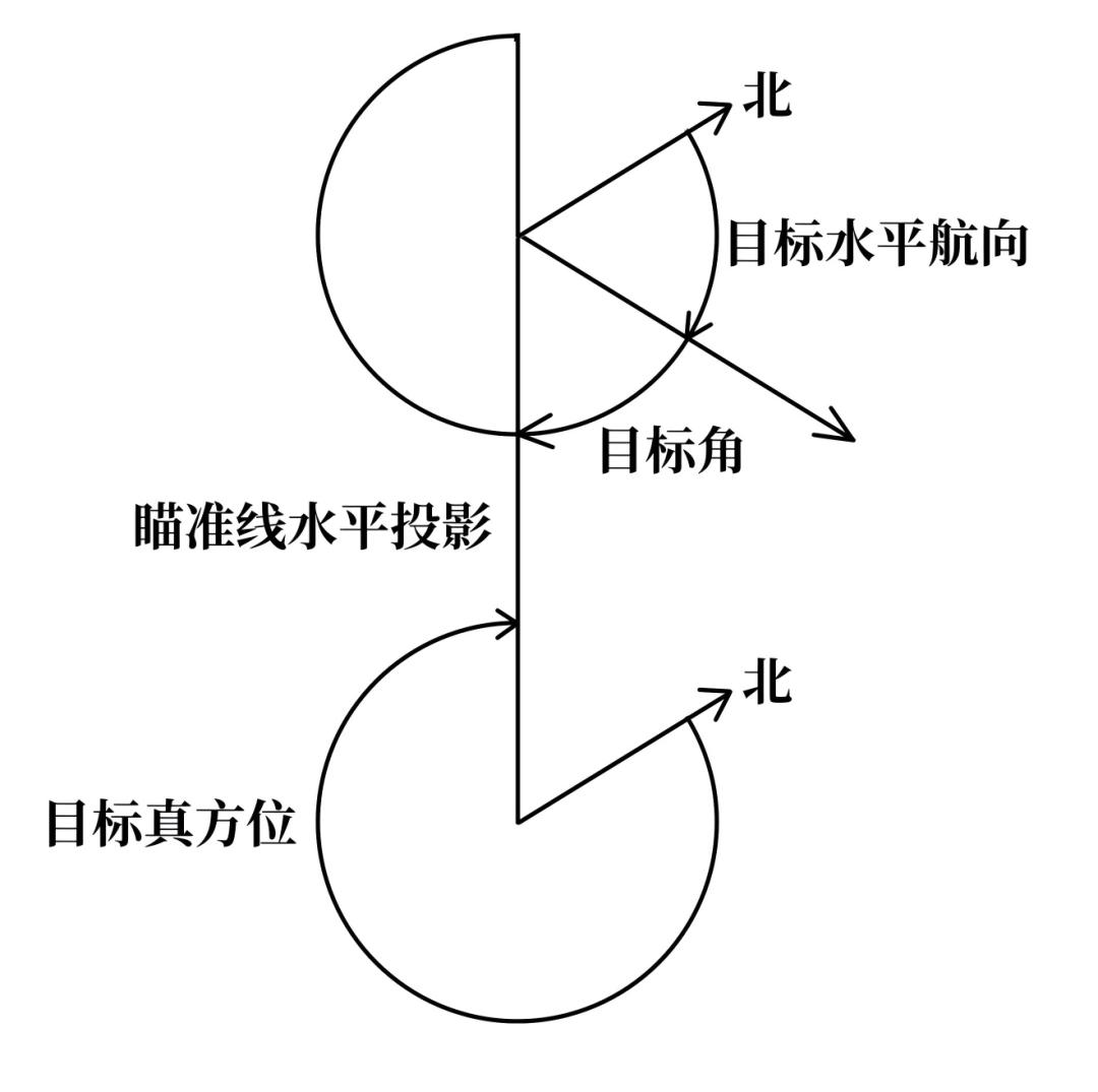
Define target angle A as the angle measured clockwise from the horizontal projection of the target’s course to the horizontal projection of the line of sight.
With the target’s horizontal velocity component Sh′ and target angle A:
horizontal range rate = −Sh′ × cosA
horizontal bearing linear velocity = Sh′ × sinA
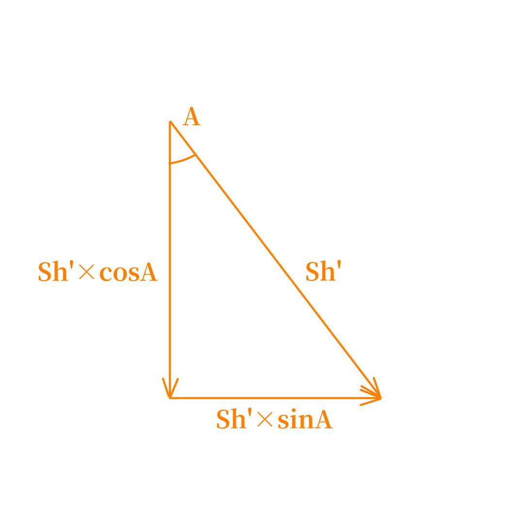
The minus sign on horizontal range rate is required by the geometry. For 0° < A < 90°, cosA is positive but the target is closing along the line of sight’s horizontal projection, so the horizontal range rate is negative. For 90° < A < 270°, cosA is negative but the target is opening, so the rate is positive. For 270° < A < 360°, cosA is again positive and the target is closing again.
The same result follows from the reduction formulas. At target angle A, Sh′ projects onto the positive range direction as Sh′ × cos(180° − A) and onto the positive bearing direction as Sh′ × sin(180° − A). Since sin(180° − A) = sinA and cos(180° − A) = −cosA, the two projections are −Sh′ × cosA and Sh′ × sinA.
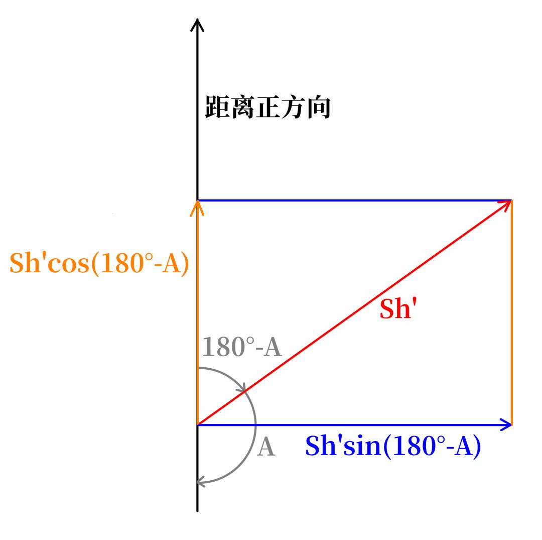
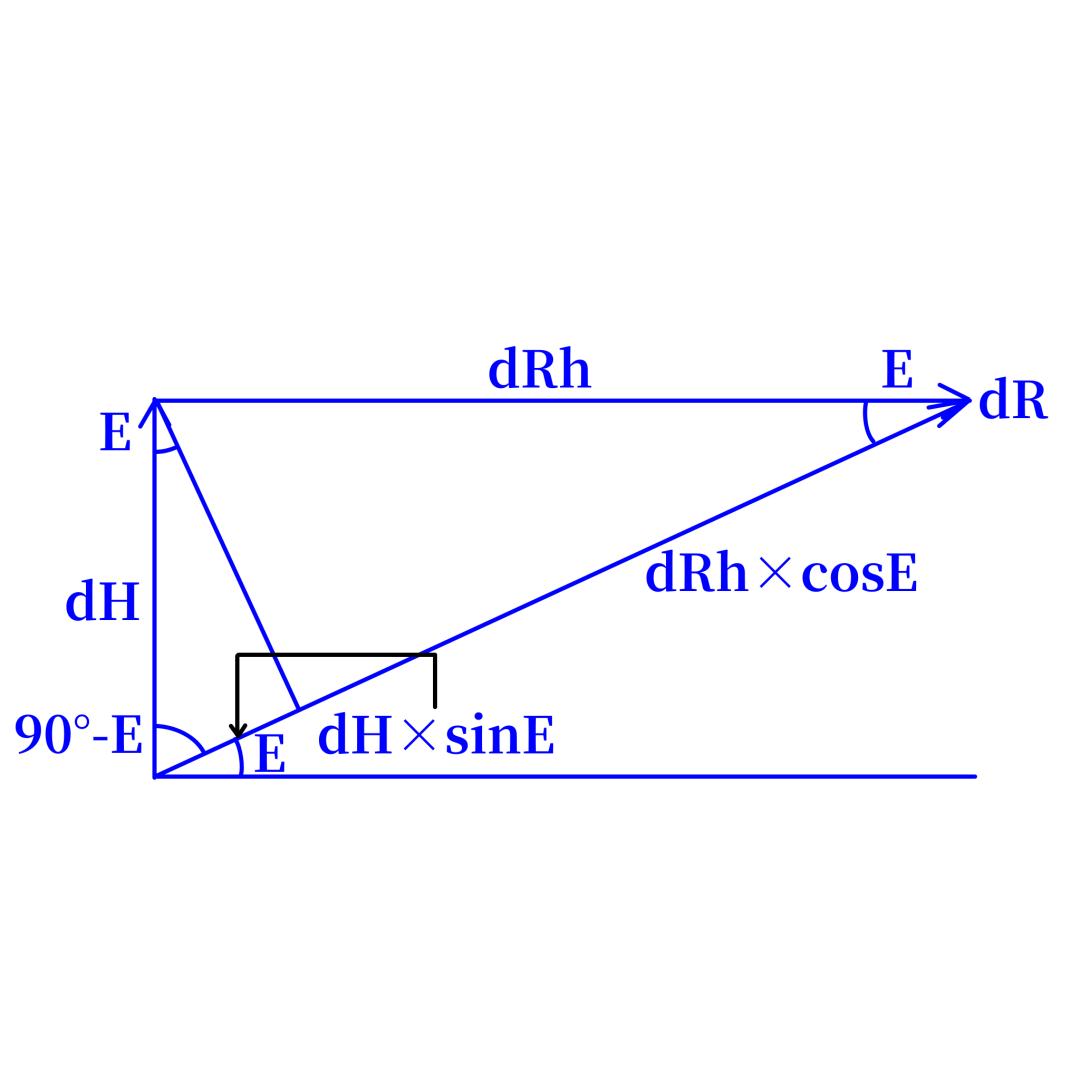
Sh′ × sinA is simply Bc′. But Ec′ and dR′ also have horizontal components. With elevation E:
Ec′ horizontal component: −Ec′ × sinE
dR′ horizontal component: dR′ × cosE
Therefore −Sh′ × cosA = −Ec′ × sinE + dR′ × cosE. The negative sign on Ec′ × sinE appears because Ec′ is positive upward, while for 0° < E < 90° its horizontal component points toward the ship and therefore shortens horizontal range. Setting −Sh′ × cosA = dRh′:
Bc′ = Sh′ × sinA (1)
dRh′ = −Ec′ × sinE + dR′ × cosE (2)
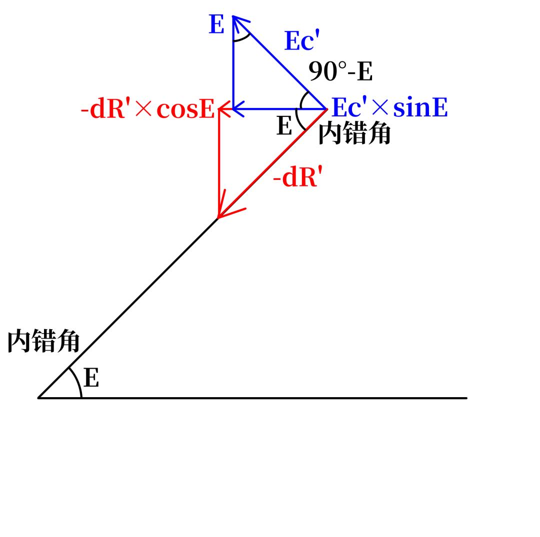
Now jBc, jEc, jdR and E are all known, so the difference jSh between the horizontal speed the computer holds and the true Sh′ follows directly:
jBc = jSh × sinA (1)
−jSh × cosA = −jEc × sinE + jdR × cosE (2)
Set −jSh × cosA = jdRh. With those parameters known the system is solvable. The question is how the MK1A solves it mechanically.
Finding Target Angle A
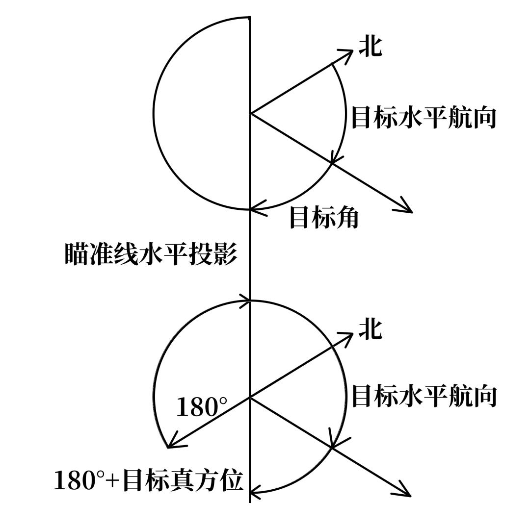
From the geometry, target angle A equals 180° + B (true target bearing) − Ct (target’s horizontal course). When the computer starts, a drive motor spins the Ct output shaft at high speed so the computer sweeps through Ct values. Because B is observable — it equals own-ship course plus relative target bearing — the quantity 180° + B − Ct sweeps just as fast. The sweep exists to prevent the assumed target angle A from landing in the wrong quadrant, which would reverse the direction of correction.
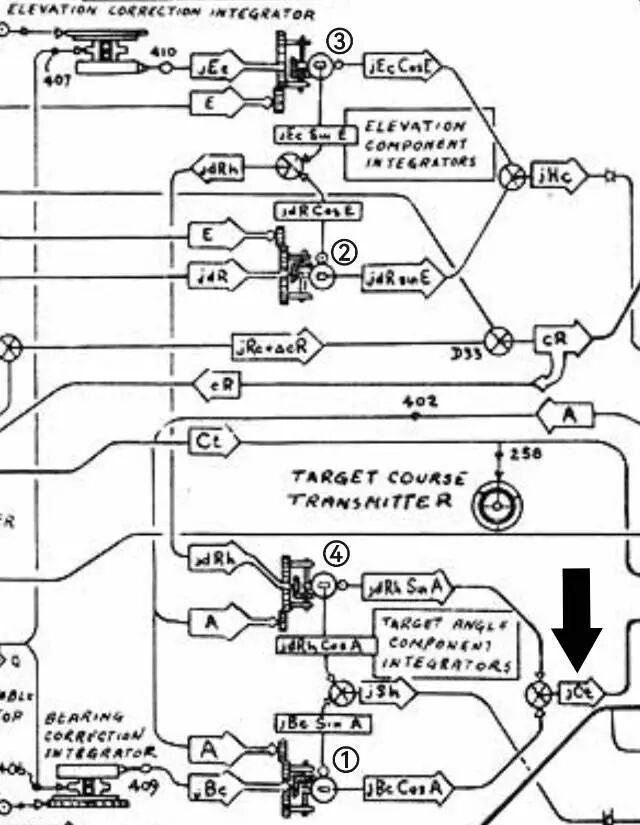
This is where a very unusual integrator enters: the component integrator.
The component integrator is a wheel-ball type, structurally much like the trackball of a computer mouse.
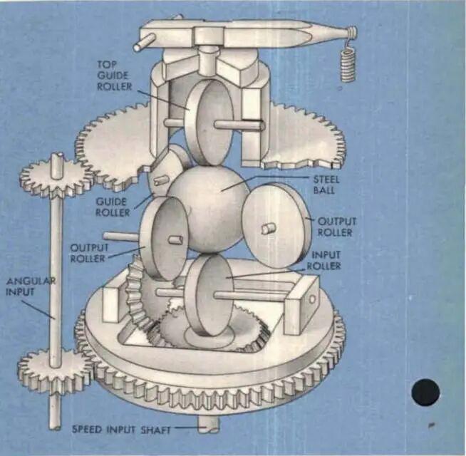
A hardened steel ball sits at the centre. A friction wheel touches it at the top and another at the bottom; the lower wheel is the driver, the upper is the guide. When the driver turns, the ball rotates in the driver’s plane. The output wheel touches the ball at its side, so once the ball is spun by the driver, it drags the output wheel around and a rotation signal appears at the output.
The odd geometry has a purpose: as the output wheel orbits the ball, the linear velocity at every point of its orbit is different. Taking the ball’s great circle in the driver’s plane — call it the meridian circle — the further to either side the output wheel sits, the smaller the ball circle it touches. Those circle radii depend on the angle the output wheel has turned through. If the output wheel starts coplanar with the driver, then after it orbits θ degrees, the circle it touches has radius Rcosθ, where R is the ball radius. If the output wheel starts perpendicular to the driver’s plane, the radius becomes Rsinθ. In other words, with the ball spinning at angular velocity ω, a coplanar output wheel delivers ωRcosθ and a perpendicular output wheel delivers ωRsinθ.
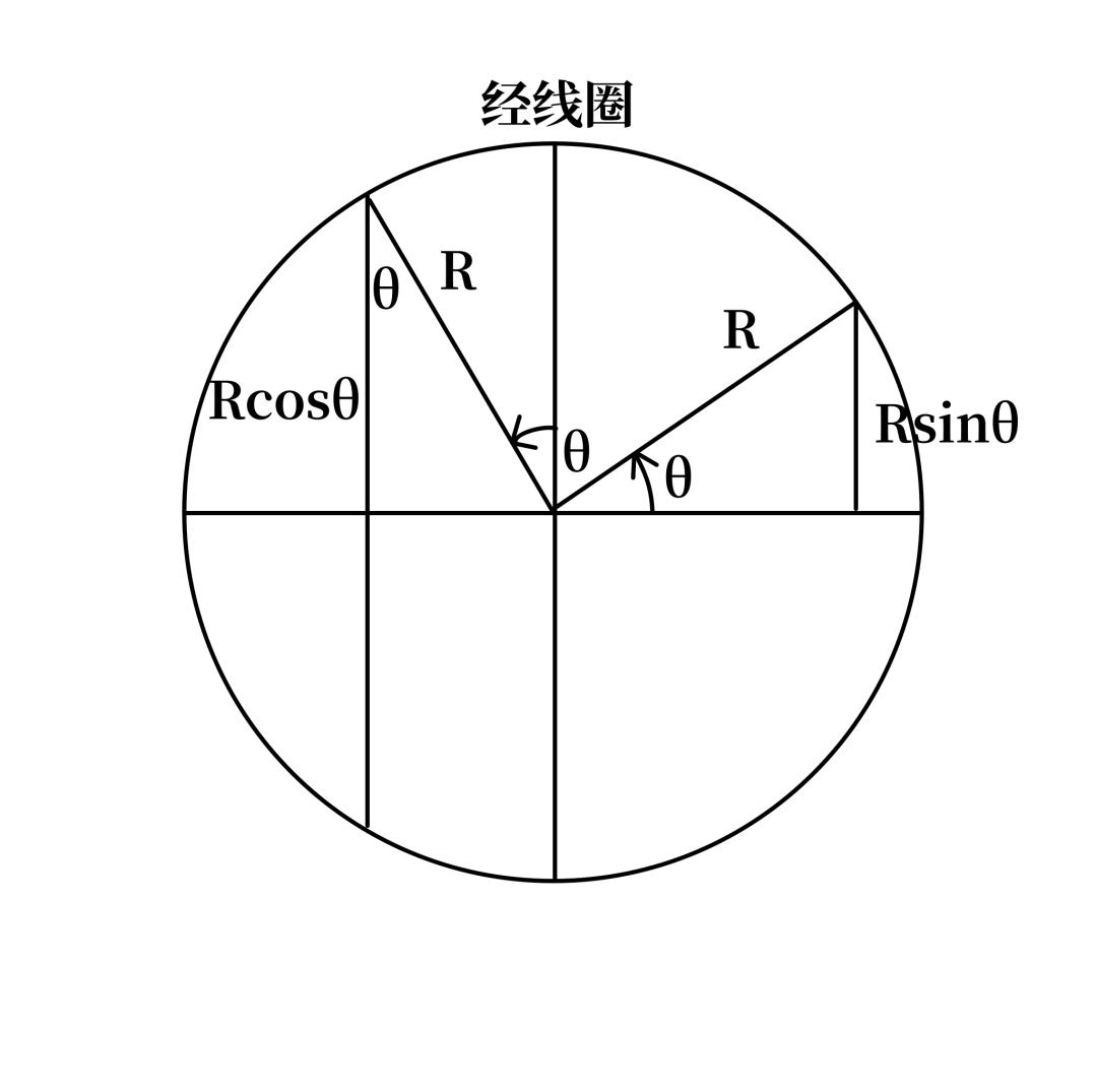
Why does that matter? Because jSh can be written another way.
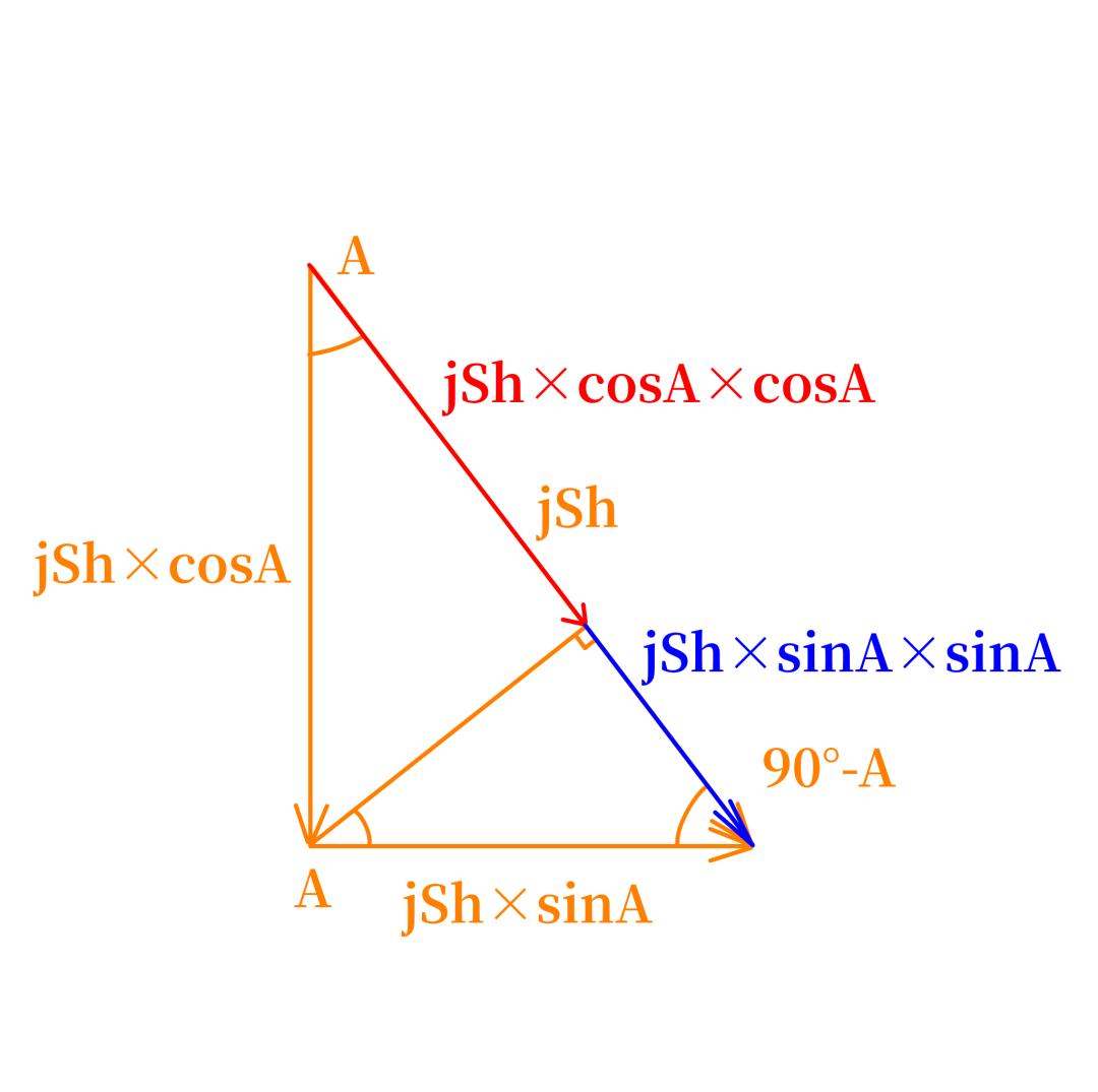
jSh also equals jSh × sinA × sinA + jSh × cosA × cosA, which is jBc × sinA + [−(jdR × cosE − jEc × sinE) × cosA] — and that expression contains both sine and cosine values.
The jBc speed from the bearing correction integrator therefore drives the ball of one component integrator, while A drives its output wheel around the ball, producing jBc × sinA. Separately, jdR and jEc each drive the ball of a component integrator while E drives their output wheels, producing jdR × cosE and jEc × sinE. Those two outputs are subtracted in a differential to give (jdR × cosE − jEc × sinE), namely jdRh. That jdRh then drives the ball of a fourth component integrator, whose output wheel is positioned by A, producing jdRh × cosA. Subtract the first component integrator’s output from the fourth’s and you have jBc × sinA − jdRh × cosA, which is jSh.
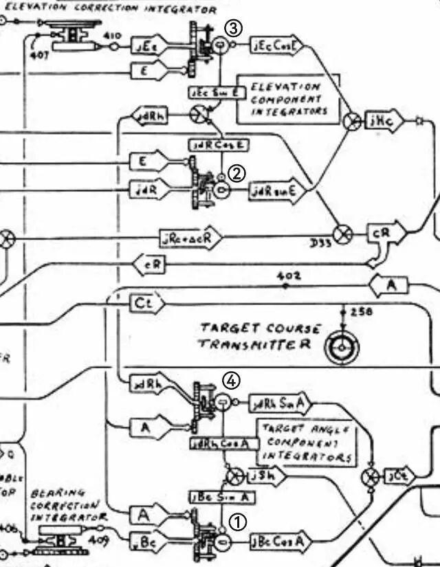
The computer now holds the difference between its own horizontal target speed Sh and the true Sh′. That jSh drives the jSh follow-up motor, which pulls the computer’s Sh toward Sh′. As the Sh shaft turns, the target speed inside the target vector resolver changes, and that change alters the resolver’s Yt output — the component of horizontal target velocity along the line of sight.
Solving for Vertical Motion
The second and third component integrators have a second output group, and it governs the vertical component of target velocity, jHc:
jHc = jEc × cosE + jdR × sinE
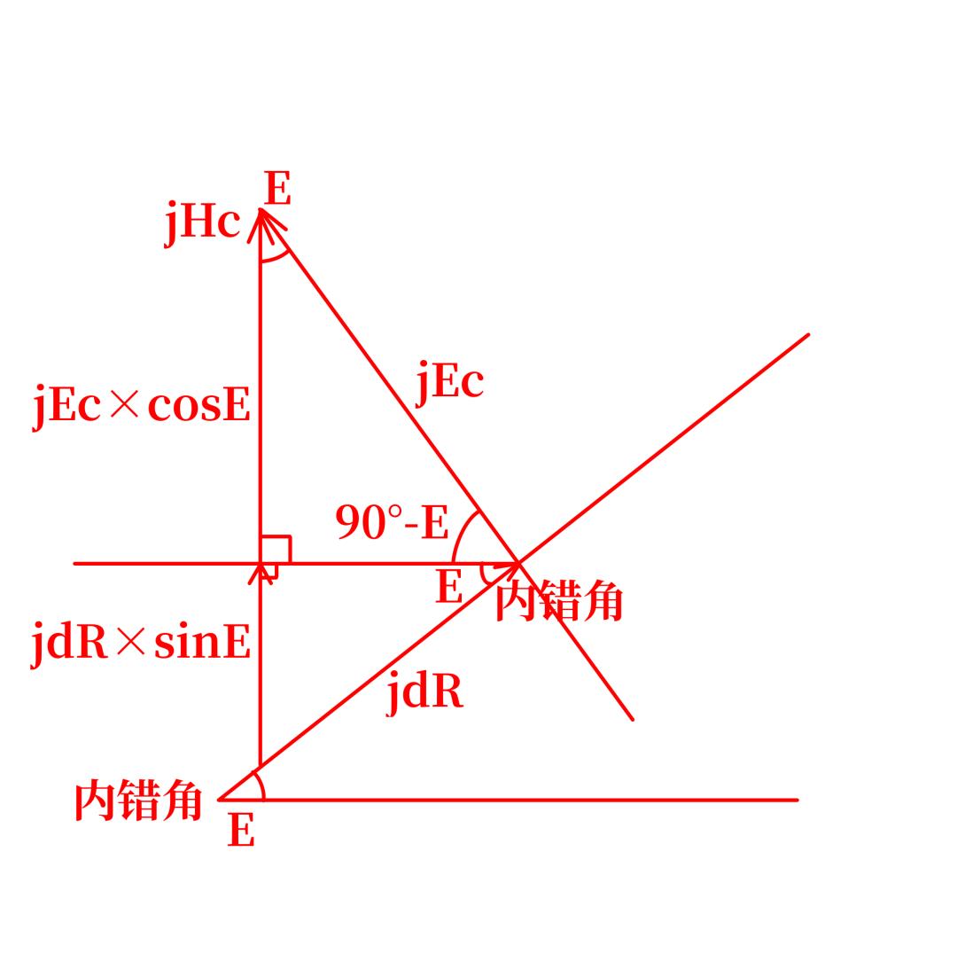
The two component integrators output jdR × sinE and jEc × cosE respectively. Fed into a differential, they sum to jEc × cosE + jdR × sinE, which is jHc. That drives the jHc follow-up motor, bringing the computer’s vertical speed dH toward the true dH′. The updated dH then enters the vertical-speed input of the height vector resolver, changing its dH × sinE output.
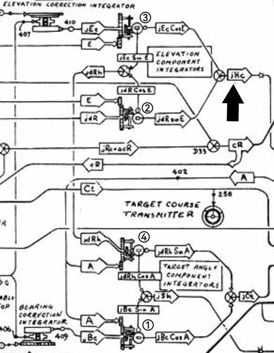
Add the own-ship velocity component along the line of sight Yo to Yt and you have the horizontal range rate dRh. Multiply dRh by cosE, add dH × sinE, and you have the target’s range rate along the line of sight, dR. Setting dR into the friction-ball position of the range ball-disc integrator changes the speed of the cR signal it outputs. As the range rate represented by that signal approaches the true one, the speed difference between the R and cR signals shrinks, and so does the jdR assist needed to make cR keep up with R. When the two speeds match exactly, the inner dial of the range dial group tracks the outer dial with no assist at all, the slip-ring switch never displaces, the jdR follow-up motor stays de-energised, and the jdR input vanishes. The computer has now fitted the target’s range rate.
Fitting Target Course Without Dividing by jSh
The assumption so far was that A is correct — that the computer started with an A matching reality. Often it does not. In that case, besides jSh, the target vector acquires a component jCt1 perpendicular to the assumed horizontal course, which rotates the course toward the true one. From the geometry, jCt1 = jBc × cosA − (−jdRh × sinA), that is jBc × cosA + jdRh × sinA.
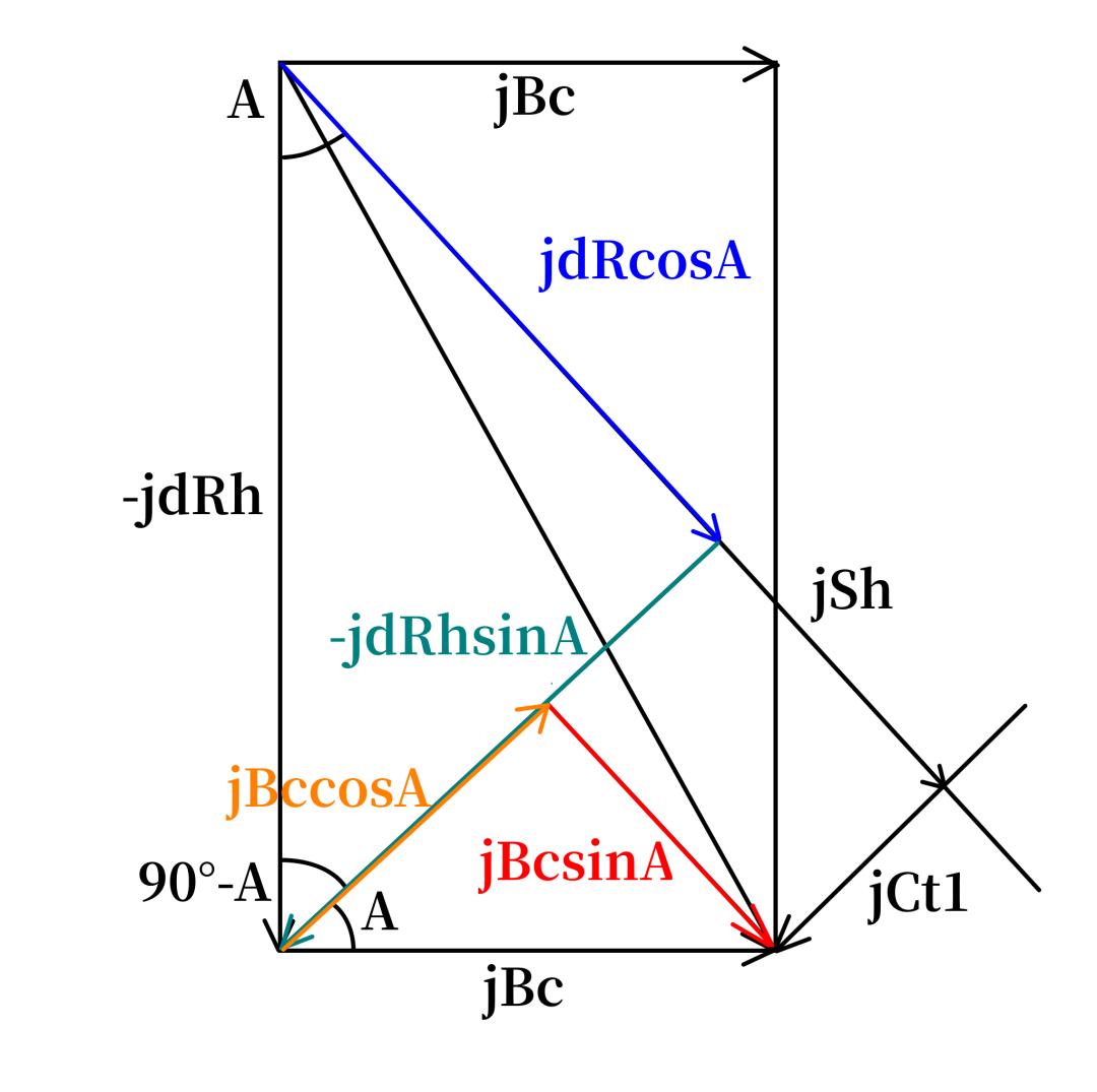
The problem is that jCt1 is a linear velocity, while correcting A to A′ requires an angle. In principle one would then compute:
arctan(jCt1 × t / jSh × t) = arctan(jCt1 / jSh)
That is the required course change jCt. It is also far too complicated to implement mechanically. So simplify it.
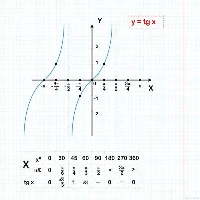
For very small angles in radians, tanθ ≈ θ. If target angle A changes by jCt in unit time and jCt is small:
tan jCt = jCt1 / jSh ≈ jCt
One awkward term remains: jSh is a variable. Making it participate would require feeding the jSh rotation signal — itself the difference of the first and fourth component integrator outputs — back into the loop, which adds real mechanical complexity.
Consider a scenario instead. Set jCt1 = 1 knot and evaluate jCt in radians for five values of jSh:
| jSh (knots) | jCt (radians) |
|---|---|
| 200 | ≈ 0.005 |
| 250 | ≈ 0.004 |
| 300 | ≈ 0.003 |
| 350 | ≈ 0.003 |
| 400 | ≈ 0.0025 |
Even a 50-knot swing in jSh moves jCt by less than 0.001 rad. There is therefore no need to use jSh at all: a fixed gear ratio K can be set so that jCt = jCt1 / K, with a final gear pair converting radians to degrees.
That is how the MK1A solves for horizontal course. Within the first and fourth component integrators there is another output group: the first outputs jBc × cosA and the fourth outputs jdRh × sinA. Summed in a differential, they give jCt1, which a gear ratio converts into jCt and drives the jCt follow-up motor, correcting the computer’s Ct toward the true Ct′. As the motor turns, its Ct signal enters differential D41, where it is subtracted from true target bearing to yield the true target angle A′ = 180° + B − Ct. The A value is continuously set into the target vector resolver’s target-angle input, so when Ct reaches Ct′ the resolver’s target angle equals A′ exactly.
With Ct′ established, the resolver’s Xt output changes accordingly — the component of horizontal target velocity perpendicular to the line of sight. Setting that bearing linear velocity Bc′ (RdBs) into the friction-ball pair of the bearing ball-disc integrator changes the integrator’s cBr output speed, so cBr chases Br until the two match, the contact switch stops displacing, and the jBr follow-up motor stops assisting. The target’s horizontal course has been formally obtained.
Fitting the Elevation Rate
The target’s velocity has more than a horizontal bearing component; it also has an elevation component in the vertical plane.
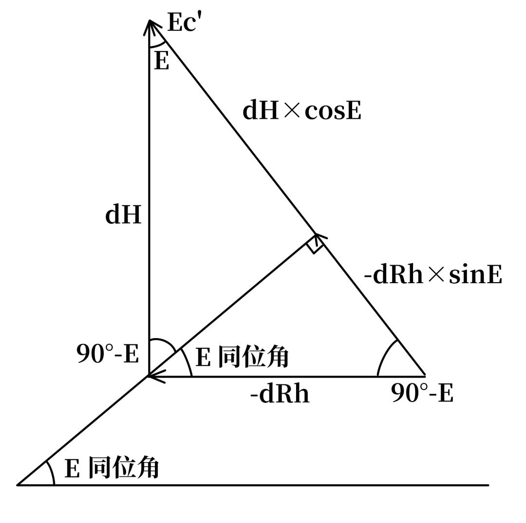
The true elevation linear velocity Ec′ can be written as (−dRh × sinE + dH × cosE). The dH and dRh values already obtained therefore produce two further outputs, dH × cosE and dRh × sinE. Subtracted in differential D31, they give the true Ec′ (RdE).
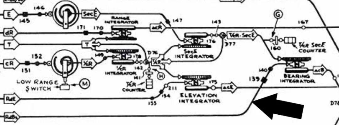
That RdE value sets the friction-ball pair of an elevation ball-disc integrator. Because the elevation integrator’s drive speed comes from a ball-disc variable-speed unit set by a reciprocal mapping disc, the drive speed is inversely proportional to range — equivalent to dividing RdE by R and applying ω = v/R to obtain the target’s elevation angular rate. The computer’s cE speed then chases E. When the two match exactly, the shafts stay synchronised, the contact switch stops displacing, the jE follow-up motor stops, and the target’s elevation linear velocity is formally obtained.
What the Three Channels Do, Side by Side
| Component | Symbol | Quantity it changes | Positive direction | Deviation pick-off |
|---|---|---|---|---|
| Bearing linear velocity | Bc (RdBs) | Target’s relative bearing | Right | Differential D39 driven by cBr and Br |
| Elevation linear velocity | Ec (RdE) | Target’s relative elevation | Up | Elevation differential, D31 |
| Rate of range change | dR | Target’s range | Opening | Slip-ring switch on the range dial group |
Why Ten Seconds Was Enough
This is how the MK1A fire-control computer fits target motion parameters without knowing the target’s motion geometry in advance. It removes the laborious manual correction process and suits the fast tempo of anti-aircraft action.
According to OP1064, with the 2-second basic time-constant gear engaged, a target inside 8,000 yards requires only 10 seconds of steady tracking to bring the fitted motion parameters to a satisfactory level — reducing the error to roughly 0.675% of its original value. That is very likely why the Royal Navy chose the MK1A over its own designs.
Have questions about this article? Feel free to contact us at [email protected] — we’re happy to help!
Frequently Asked Questions
What did the MK1A fire-control computer actually do?
It continuously fitted a target’s course, speed and rate of range change from tracking observations alone, then produced the gun orders needed to intercept. It removed the manual correction step that earlier systems required from the director crew.
Why did HMS Vanguard carry an American computer instead of a British one?
Because the MK1A proved more capable than contemporary British designs. It was already the standard heavy anti-aircraft computer across the US fleet, from destroyers to battleships, and it stayed in service through the Cold War, including aboard the Iowa class.
How long does the MK1A take to settle on a target’s motion?
About 10 seconds of steady tracking. With the 2-second basic time-constant gear fitted, targets inside 8,000 yards converge to within roughly 0.675% of the initial parameter error, per the OP1064 manual.
What is a component integrator and why is it shaped like a trackball?
It is a wheel-ball integrator whose output wheel orbits a steel ball. Because the ball circle under the output wheel scales as Rcosθ or Rsinθ, one mechanical unit can multiply a rate by a sine or cosine — which is exactly what resolving a velocity vector requires.
How does the MK1A measure a target’s motion error without radar?
By differencing two rates. The director supplies the observed bearing, the computer supplies its own predicted bearing, and a differential compares the two shaft speeds. The resulting error drives a follow-up motor, whose speed is held equal to the error by pulsing regulation.
About Aomway
Aomway has been developing and manufacturing video transmission and UAV radio hardware for over 15 years, producing equipment for any frequency band from 1 GHz to 9 GHz at power levels from 3W to 15W. We build high-power FPV video transmitters, directional and circularly polarised antennas, digital links, fiber-optic tether systems and detection hardware for pilots, integrators and commercial operators worldwide.