

Key Takeaways
- Eight random seeds all hit, with miss distance between 18.705 m and 19.937 m against a 20 m threshold, which is a marginal intercept.
- The configured 850 m/s speed ceiling was never reached: 1200 N of thrust balances drag at about 442 m/s.
- A wrong EKF prediction step of 0.01 s against a real 0.02 s cycle doubled the speed estimate and produced a 1088 m miss.
- Pure pursuit diverged to over 100 deg/s line-of-sight rate at the endgame; proportional navigation fixed it structurally, not by tuning.
Missile intercept simulation in this project is a single-file MATLAB build that chases an actively evading aircraft using only noisy seeker measurements, and it went from a 1088 m miss to 8 out of 8 seeds hitting in 2026. The interesting part is not the final number but the two structural bugs that had to be found first: a filter whose time base was wrong by a factor of two, and a guidance law that diverges by construction against a crossing target.
Start with an uncomfortable fact
Suppose you are an air-to-air missile closing on a fighter at 850 m/s. The pilot spots you at 12 km and pulls 6 g into a rolling evasive turn, which means his body is carrying six times its own weight and his vision is starting to grey out. You have 20 g to spend, so you should have the advantage.
The opposite is true. In this replication, 20 g at 850 m/s buys a turn rate of only about 13.2 deg/s, while the aircraft pulling 6 g at 250 m/s turns at about 13.5 deg/s, which is faster than you. That is the real dilemma of the air-to-air missile: the faster you fly, the wider your turn radius. You outrun your opponent but you out-turn him less. In the last few seconds, whoever can bite into the error first wins.
This article documents the full build of that scenario as a runnable three-dimensional simulation, including the ten traps hit along the way.
What the replication has to achieve
The goal in one sentence: make a missile chase an aircraft that is actively evading it, using only noisy radar measurements plus its own estimate of where the target is.
The difficulty is in the parenthesis. The missile is not allowed to know the aircraft’s true coordinates, because that would be cheating. Every 0.02 s it receives one measurement set from the seeker, consisting of range, azimuth and elevation, and those measurements carry noise: 20 m in range and 1 degree in each angle. From that it has to infer where the aircraft is and how fast it is moving.
That inference process is the Kalman filter.
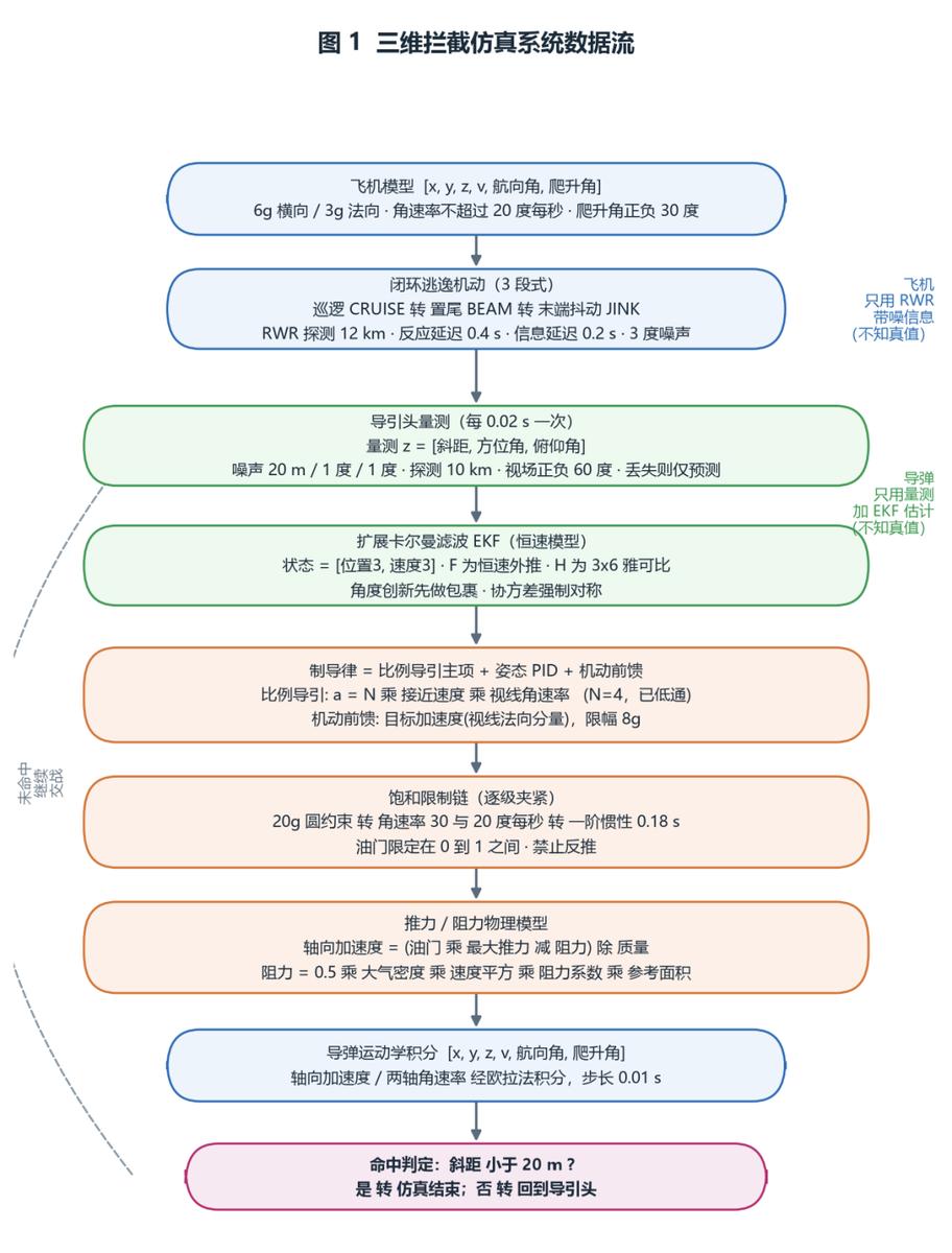
The data flow runs as follows: the aircraft flies a closed-loop evasive manoeuvre, the seeker returns only noisy range and angles, an extended Kalman filter estimates the target state, proportional navigation turns that into load factor and throttle commands, and saturation limits are applied before the kinematics integrate. The key annotation on both sides is that neither vehicle ever gets the other’s ground truth.
Three physical constraints that cannot be avoided
Three facts set the entire difficulty of the problem.
Constraint 1: you cannot turn just because you want to
How fast an object can turn is inversely proportional to its speed:
turn rate = available load factor x gravitational acceleration / speed
Read it plainly: with load factor fixed, doubling speed halves the angular rate you can generate. Substituting the real parameters from the code:
| Vehicle | Available load factor | Speed | Turn rate available |
|---|---|---|---|
| Aircraft (F-16 class) | 6 g | 250 m/s | About 13.5 deg/s |
| Missile (AIM-9 class) | 20 g | 850 m/s | About 13.2 deg/s |
| Same missile | 20 g | 442 m/s | About 25.4 deg/s |
The third row is the important one: dropping the missile from 850 to 442 m/s doubles its turning ability. That is why speed was later treated as a tunable quantity rather than something to maximise, and that reframing rescues the design later on.
Constraint 2: if you cannot see it, it does not exist
The seeker has a field-of-view cone: it only sees the target within plus or minus 60 degrees of the missile’s nose. It is like looking out through a very wide pipe, and anything outside the pipe simply is not there. The problem is that during a hard turn the body attitude and the line of sight diverge. In the worst variant of this replication the off-boresight angle reached 117 degrees, far outside the field of view, and the lock rate fell to 74 percent.
Worse, there is a positive feedback loop: cannot see, so it can only predict; prediction error grows, so it falls further behind; falling further behind means it sees the target even less.
Constraint 3: more speed is not better
The missile uses a real thrust and drag model rather than a speed set directly:
axial acceleration = (throttle x max thrust – aerodynamic drag) / mass
aerodynamic drag = 0.5 x air density x speed squared x drag coefficient x reference area
Throttle runs between 0 and 1, so it can only reduce thrust and never produce reverse thrust. The only way to slow down is to close the throttle and let drag pull the speed down, and drag grows with the square of speed.
It is like flooring a car: air resistance rises with it and the speed settles at an equilibrium point. Not because you do not want to go faster, but because physics will not let you. Measured, the missile’s actual speed envelope was 300 to 442 m/s with a mean of 375, and the configured 850 m/s ceiling was never touched once. That finding produces an awkward conclusion, covered later.
The build: ten traps, two real problems
The environment was MATLAB R2023b using only base functions, with no toolbox dependency. Even wrapToPi was reimplemented by hand because it belongs to the Mapping Toolbox.
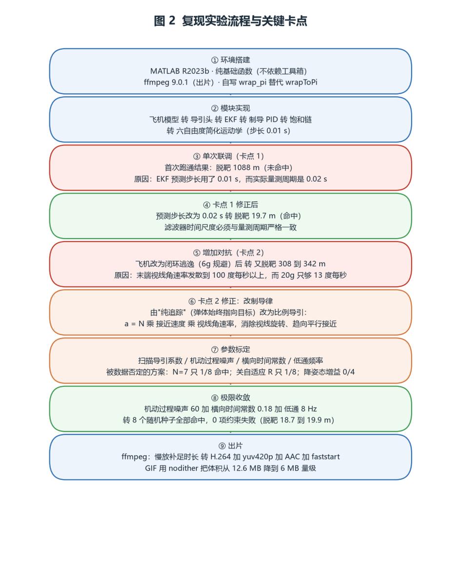
The replication follows the real timeline across nine stages. There were two genuine failures: the filter prediction step was wrong, producing a 1088 m miss, and once closed-loop evasion was added the original guidance law lacked endgame authority, producing misses of 308 to 342 m. Both were model and algorithm errors, not tuning problems.
Environment
MATLAB R2023b, a single-file script with local functions, more than 40 functions and about 140,000 bytes. ffmpeg 9.0.1 was added separately so the animation could be rendered to video.
Trap 1: a 1088 m miss that was not a parameter problem
Symptom: the first successful run missed, with a miss distance of 1088 m, and the Kalman filter’s velocity estimate error reached 258 m/s while the target aircraft was only flying at 250 m/s.
Diagnosis: that number was too suspicious. An error of 258 m/s mapping almost one to one onto the target’s own speed suggested the filter was not estimating badly but estimating double. The call cadence explained it: the filter was invoked every 0.02 s, following the seeker measurement period, but the internal prediction matrix F used the simulation step of 0.01 s. The filter’s time base was therefore off by a factor of two, believing 0.01 s had passed when 0.02 s actually had. Double the time, double the velocity.
Fix: set the prediction step to pred_dt = 0.02, equal to the measurement period. The miss distance dropped immediately from 1088 m to 19.7 m and the shot hit.
Why it matters: the F matrix is not a place to put an arbitrary time. It must equal the real interval between filter invocations. This class of error throws no exception and crashes nothing; it only makes the output look slightly wrong and then stays wrong all the way to the end. Its signature is an estimation error that scales as an integer multiple of some physical quantity.
Trap 2: once the aircraft started evading, nothing hit again
The aircraft was changed to a closed-loop evasion as specified: detect the missile with the radar warning receiver, begin evading after a 0.4 s reaction delay, and run a three-phase policy of patrol, tail-away evasion that swings 90 degrees to the missile’s beam and reverses every 3.6 s to form an S-shaped weave, and terminal jinking on a 1.6 s high-frequency cycle. At the same time the missile’s speed ceiling was raised to 3.4 times the aircraft’s speed, matching the real speed ratio.
Symptom: miss distances of 308 to 342 m, every seed a miss.
Diagnosis: endgame data showed two numbers. The off-boresight angle was 117 degrees, long outside the 60 degree field of view, and the terminal line-of-sight rate diverged above 100 deg/s. Checking the physical constraint: at 850 m/s, 20 g only buys 13.2 deg/s. The requirement was 100 and the capability was 13, a factor of seven, which no tuning can close.
Asking one level deeper: why was the terminal line-of-sight rate so large? Because the guidance law was pure pursuit, which points the body straight at the target. Pure pursuit has a fatal property: when the target crosses the line of sight, the turn rate it demands tends to infinity.
It is like standing at a crossing watching a pedestrian walk past. At the instant he is directly abeam, your head would have to snap through 90 degrees. If it cannot, you lose him.
Fix: switch to proportional navigation.
load factor command = navigation constant N x closing velocity x line-of-sight rate
The law stops staring at where the target is and instead stares at how fast the sight line is rotating, driving that rotation to zero. If the sight line stops rotating, the two vehicles are on a collision course. Adding manoeuvre feedforward, which injects the estimated target acceleration into the command, plus recalibrated parameters, brought all eight random seeds to a hit.
Approaches the data rejected
Not every attempt succeeded. The following were measured, rejected and not adopted, and they are recorded because eliminating wrong options is also a result.
| Attempt | Result | Conclusion |
|---|---|---|
| Raise navigation constant N to 6 or 7 | Hit rate fell to 2/8 and 1/8 | N too large amplifies measurement noise into jitter |
| Disable adaptive measurement noise R | Hit rate fell to 1/8 | Adaptive R was retained |
| Lower attitude loop gain to 400 or 200 | 0/4 hits | Gain too low, the body stops following the target and lock is lost |
| Cap speed at 400 m/s | 0/8 hits | Slower than the target, it can never catch up |
| Reduce lateral time constant to 0.08 s | Hit rate fell to 1/8 | Response too fast triggers oscillation |
There is a counterintuitive point here. One section argues that slowing down buys manoeuvrability, while this table shows that slowing down too much loses the chase. Both are true: there is an optimal band for trading speed for manoeuvrability, and beyond it the energy deficit overwhelms the manoeuvre advantage.
Front-end traps worth listing
| Symptom | Diagnosis | Fix |
|---|---|---|
| Error: undefined field a_lat_max | Config field name did not match the reference | Unify the naming and convert to acceleration at the point of use |
| Error: los_ang not recognised | Variable referenced before it was computed | Reorder the statements |
| HUD Chinese text rendered as boxes | listfonts showed Consolas has no Chinese glyphs |
Switch to Microsoft YaHei UI |
| GIF too large at 12.6 MB with a noisy background | Dithering enabled by default during quantisation | Use nodither, size drops to about 6 MB |
| Video 10.2 s, blocked by the platform minimum | Platform requires more than 10 s | Slow it to 13.84 s in ffmpeg and shift the audio events |
| Same seed gave different results in record and silent modes | The sound synthesis random function consumed the global random stream and polluted the measurement noise sequence | Save the stream state before synthesis and restore it afterwards |
The last row deserves its own paragraph. Any module that looks unrelated can still pollute a simulation result if it shares the same random number generator. This bug made the same seed produce both a hit and a 32 m miss, and it was located only by comparing the miss distance between the two run modes.
Run it yourself
% after switching to the project folder:
missile_intercept_3d('verify')   % full run: 9 result figures + 16 constraint checks
missile_intercept_3d('quiet', 42)   % silent run of one seed, returns a metrics struct

rep = missile_intercept_3d('quiet', 42);   % rep.miss is the miss distance, rep.ck the constraint table

% parameter sweep without editing the source:
ov.ms.tau_lat = 0.15;  ov.pid.N_pn = 3.5;
r = missile_intercept_3d('quiet', 42, ov);
The engineering point is that the code needs no toolbox and no Simulink, and even wrapToPi is implemented locally. It runs on arrival with nothing installed, all parameters live in a single make_config function, and after editing you run the quiet mode for batch validation. A parameter sweep should be one automated command, not edit, rerun and stare.
Results
Regression across eight random seeds in the final configuration:
| Seed | Hit | Miss distance (m) | Intercept time (s) | Peak missile speed (m/s) | Constraint failures |
|---|---|---|---|---|---|
| 1 | Yes | 19.937 | 14.320 | 448.09 | 0 |
| 7 | Yes | 19.092 | 16.650 | 471.82 | 0 |
| 42 | Yes | 19.139 | 14.090 | 445.67 | 0 |
| 99 | Yes | 19.482 | 14.360 | 448.71 | 0 |
| 2024 | Yes | 19.586 | 13.850 | 442.20 | 0 |
| 5555 | Yes | 19.832 | 14.130 | 445.96 | 0 |
| 8888 | Yes | 19.698 | 14.260 | 447.67 | 0 |
| 12345 | Yes | 18.705 | 13.770 | 442.25 | 0 |
Eight of eight hits, zero constraint failures, miss distance between 18.705 and 19.937 m.
One honest caveat: the hit threshold is 20 m and the miss distance sits right against it. This is a marginal intercept, not a comfortable one.
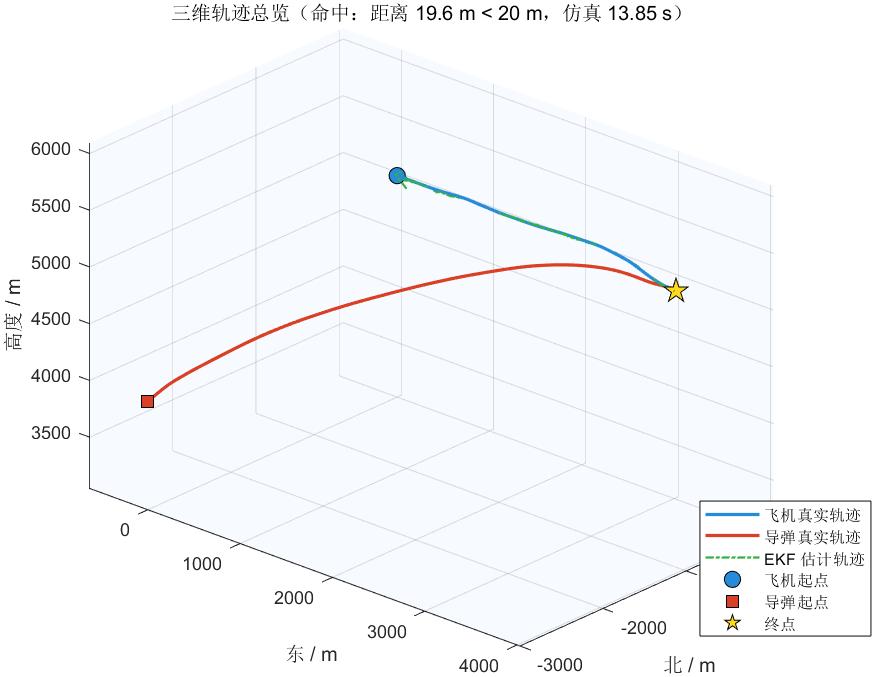
Blue is the aircraft’s true trajectory, red is the missile, and the green dash-dot line is the filtered target estimate. The missile climbs, flattens out and turns sharply at the end, and both trajectories converge on the star-shaped endpoint. The green estimate tracks the blue truth closely without ever coinciding with it, because it is an inference rather than the truth.
How good is the filter?
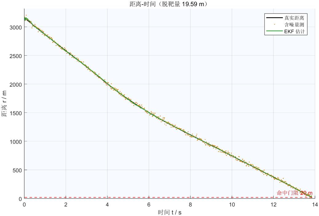
Black is true range, the yellow scatter is the seeker’s raw measurement, and the spread of that scatter is the 20 m noise made visible. Green is the filter estimate. Range falls monotonically from 3162 m to inside 20 m, and the green line passes smoothly through the scatter, which shows the filter turning partly untrustworthy measurements into a more trustworthy estimate.
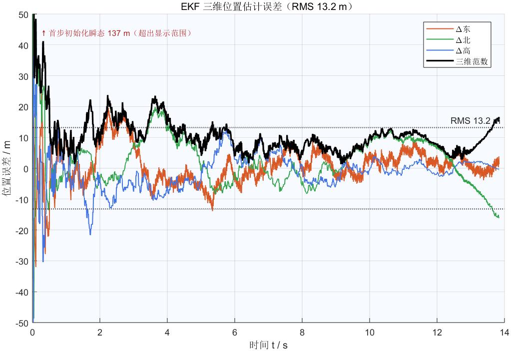
The three coloured lines are estimation error in the east, north and altitude channels, and the black line is the three-dimensional norm. Terminal position error RMS is about 13 m, better than the 20 m measurement noise level, which confirms the filter is fusing history. The velocity estimation error RMS of 49.62 m/s is large, and the reason is structural: the target sustains 6 g manoeuvres while the filter uses a constant-velocity model, so velocity lags by nature. Guidance depends on position, so this is acceptable.
Load factor and limits: are the constraints real?
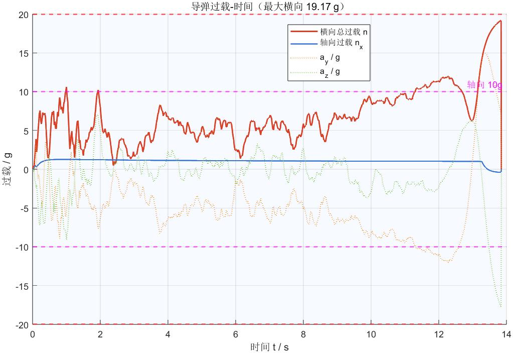
The four curves are total lateral load factor, axial load factor and the two lateral channel components. The red dashed line is the 20 g circular constraint and the magenta dashed line the 10 g axial boundary. Lateral load factor approaches but never crosses 20 g at the endgame, so the saturation is genuine rather than decorative. Axial load factor stays far below 10 g throughout because 1200 N of continuous thrust gives a modest thrust-to-weight ratio and acceleration is slow.
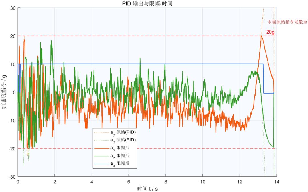
The dashed line is the raw command from the guidance law and the solid line is what was actually executed after the 20 g circular constraint and the angular-rate limit. Early in the engagement the two nearly coincide; at the endgame the raw command spikes and is pressed onto the 20 g boundary, which is saturation. Because saturation lowers the effective gain, anti-windup logic was added so the integral term cannot accumulate without limit while saturated.
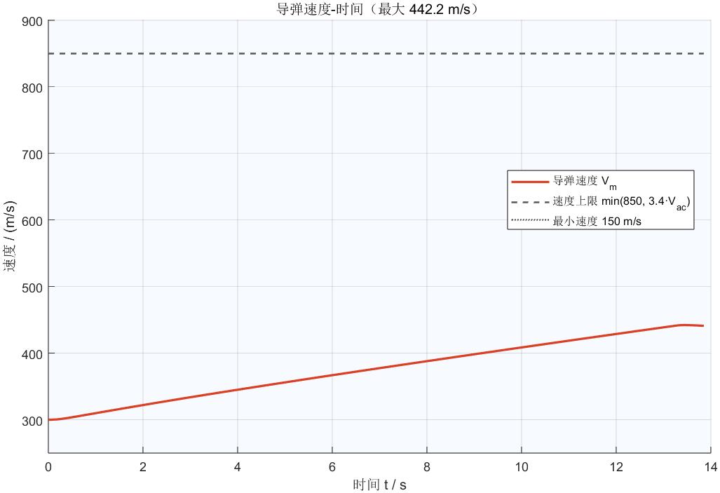
Red is the missile’s actual speed, climbing from 300 m/s and flattening near 442 m/s where thrust and drag balance. The dark dashed line is the configured 850 m/s ceiling, and actual speed never came near it. This is not a bug but the inevitable result of a real drag model: drag grows with the square of speed, so 1200 N only pushes the missile to 442 m/s.
How the aircraft evades
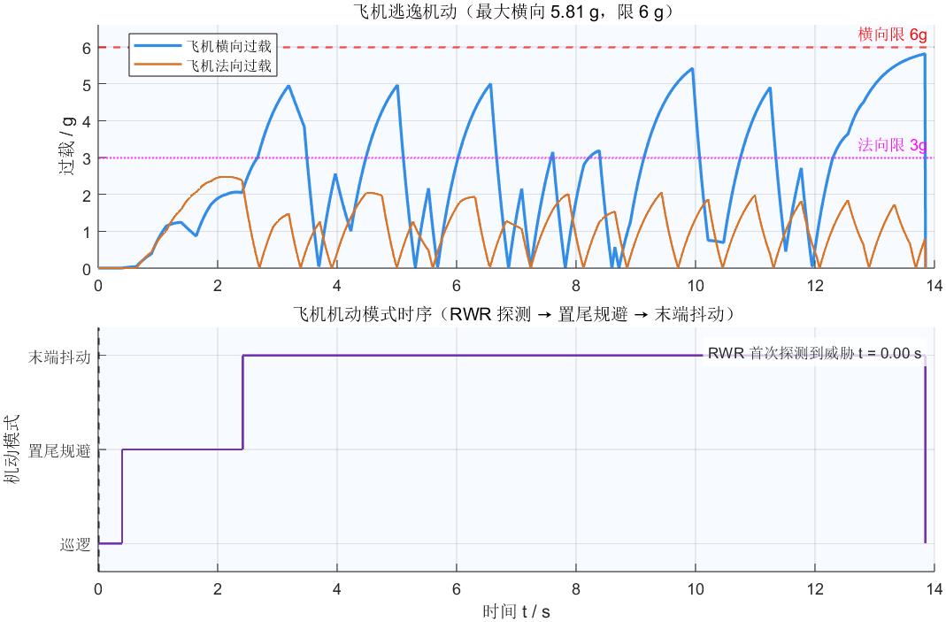
The upper plot is the aircraft’s lateral and normal load factor with 6 g and 3 g limit lines. The lower plot is the manoeuvre mode staircase: the threat is detected at 0 s, the aircraft keeps patrolling for the first 0.4 s as reaction delay, then transitions to tail-away evasion, and spends the last 82.5 percent of the time in terminal jinking. Peak lateral load factor is 5.988 g, just 0.012 g short of the 6 g ceiling, which shows it too is physically limited rather than infinitely agile.
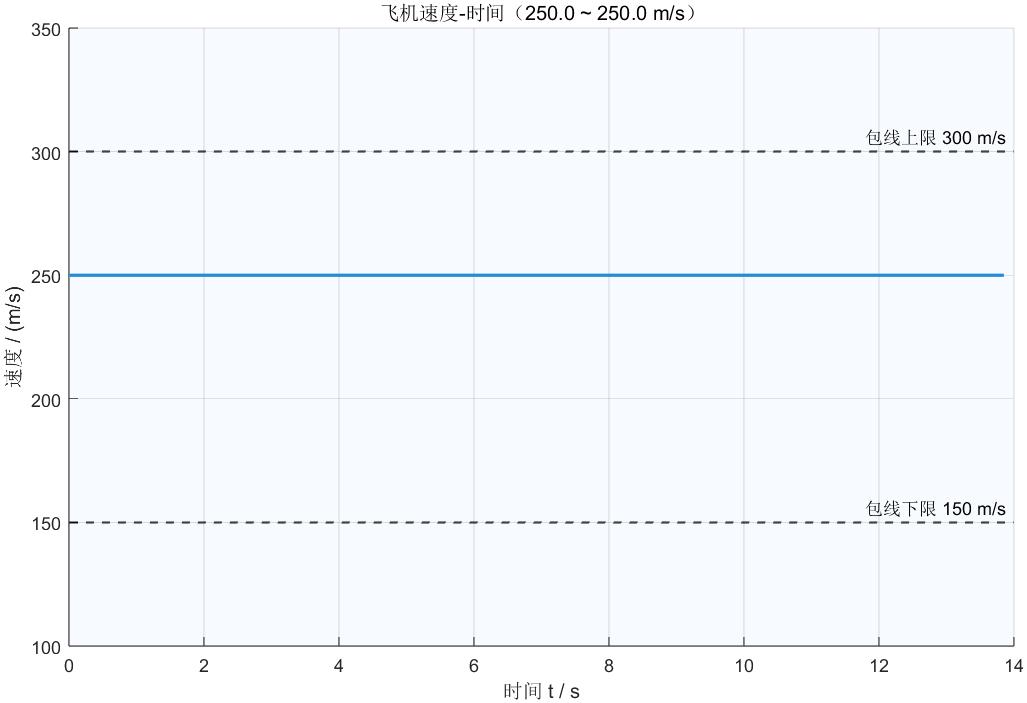
Aircraft speed holds at 250 m/s with only small ripple from first-order engine tracking, never leaving the 150 to 300 m/s envelope. That is realistic: a pilot evading prioritises turning and energy retention over large speed changes, and with information that is 0.2 s old and noisy, fine speed deception is not achievable anyway.
The awkward finding: the 2x speed constraint never engaged
A controlled experiment was run to test the requirement.
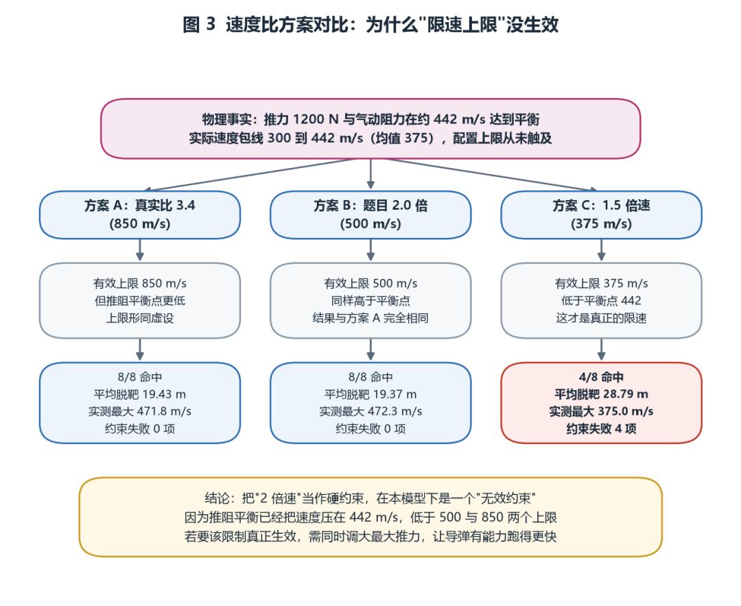
Scheme A used the real speed ratio of 3.4 and scheme B the required 2.0, and in both cases the ceiling sat above the thrust-drag equilibrium of 442 m/s, so the limit was inert and the results were identical at 8/8 hits. Only scheme C, pressed down to 1.5, actually limited speed, and it produced 4/8 hits. Whether a constraint is effective depends on whether it sits below the system’s natural equilibrium point.
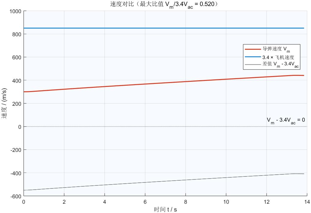
The red solid line is missile speed, the blue solid line the speed corresponding to the ratio ceiling, and the grey line the difference. Because the ceiling is far above actual speed, the difference stays negative throughout, which is the visual proof that the constraint never engaged. A strict 2x experiment would need the maximum thrust raised at the same time, so the missile could first reach 500 m/s or more.
The finding changed the wording of the write-up: instead of claiming that a 2x speed constraint was implemented, the honest statement is that the constraint was verified not to constitute an effective boundary under the current physical model. The latter is what the simulation actually established.
Three takeaways
Speed is double-edged, and manoeuvrability decides the endgame
Turn rate equals available load factor times gravitational acceleration divided by speed. The missile was 1.8 times faster than its target but had only 3.3 times the available load factor, so speed ate the manoeuvre advantage. What decides a hit in the last few seconds is not who is faster but who can turn harder in the final 500 m. The same logic transfers to drone interception, missile defence and even racing through a corner: energy management is not about maximising energy but about converting it into the manoeuvrability you need at the moment you need it.
Pure pursuit fails against a manoeuvring target, and it is not a tuning problem
Pointing the body at the target sounds like the most natural choice, but the turn rate it demands tends to infinity when the target crosses the line of sight. That is a structural defect and no parameter will save it. The fix is proportional navigation: stop pointing at the target and start nulling the rotation of the sight line, which converts a diverging terminal line-of-sight rate of over 100 deg/s into a converging one. The general lesson is that when a control problem hits a physical ceiling, check whether the objective is wrong before reaching for more gain.
The worst traps hide in places that look unrelated
The two most covert bugs were a prediction step of 0.01 s against a real 0.02 s cycle, which doubled the velocity estimate and cost 1088 m, and a sound module consuming random numbers that polluted the measurement noise sequence, which made the same seed produce both a hit and a 32 m miss. Neither threw an error or crashed anything; both only made the results look slightly odd. The method for finding them is the same: pick a quantity that should have no correlation and check whether it shows one, such as a velocity error exactly equal to the target speed, or two run modes that should agree but do not.
An open question
The results section states plainly that miss distance runs from 18.7 to 19.9 m against a 20 m threshold. That is a marginal bite, not a comfortable margin. So the question is: in a real engagement, where would you spend the resources?
- A. Raise the missile’s load factor ceiling from 20 g to 30 g, at the cost of structural weight.
- B. Lower the terminal engagement speed, trading speed for manoeuvrability, at the cost of possibly being unable to catch up when energy is short.
- C. Improve seeker field of view and counter-countermeasures to reduce lock loss, at the cost of money and weight.
The measured data leans toward B: dropping from 850 to 442 m/s turned a total miss into 8/8. But B has a boundary too, and pressing down to 375 m/s produced 4/8. Where the optimum sits is an open question.
Have questions about this article? Feel free to contact us at [email protected] — we’re happy to help!
Frequently Asked Questions
What was the final hit rate of this missile intercept simulation?
Eight of eight random seeds hit, with miss distance between 18.705 m and 19.937 m against a 20 m threshold and zero constraint failures. The author describes it as a marginal intercept rather than a comfortable one.
Why did the missile miss by 1088 m on the first run?
The Kalman filter’s prediction matrix used a 0.01 s step while the filter was actually called every 0.02 s. The time base was off by a factor of two, so the velocity estimate doubled. Setting the step to 0.02 s dropped the miss distance to 19.7 m.
Why did pure pursuit fail against an evading aircraft?
Pure pursuit demands a turn rate that tends to infinity when the target crosses the line of sight. At 850 m/s and 20 g the missile could generate only 13.2 deg/s while the endgame demanded over 100 deg/s, a sevenfold gap that tuning cannot close.
Did the missile ever reach its 850 m/s speed ceiling?
No. With 1200 N of thrust, aerodynamic drag balances at about 442 m/s, so actual speed ranged from 300 to 442 m/s with a mean of 375. The configured ceiling was never approached, which is why the 2x speed constraint had no effect.
Why is the EKF velocity error so large at 49.62 m/s?
Because the target sustains 6 g manoeuvres while the filter uses a constant-velocity model, so velocity inherently lags. Position error RMS is about 13 m, better than the 20 m measurement noise, and guidance depends on position, so the velocity lag is tolerable.
About Aomway
Aomway is a radio-frequency engineering company that designs and manufactures long-range FPV video transmitters, antennas, goggles and UAV communication links, and it publishes technical notes on guidance, estimation and embedded control. Its hardware is built for builders who need dependable links at range, and its documentation aims to explain the engineering behind each product.