
Key Takeaways
- This project extends a working single-antenna OFDM receiver into a 2Tx × 2Rx MIMO-OFDM system using true spatial multiplexing, not Alamouti coding — two independent 16QAM streams are transmitted at the same instant on the same subcarriers.
- Channel estimation uses two orthogonal training symbols: in the first, Tx1 transmits while Tx2 stays silent; in the second the roles swap. That yields all four coefficients of the 2×2 matrix per subcarrier without complex orthogonal sequence design.
- The expensive part of zero-forcing — the matrix inverse — is precomputed during training and stored as equalizer weights, so the payload detector only performs 4 complex multiplies and 2 complex adds per subcarrier, sustaining one subcarrier per cycle.
- Two FFT instances are mandatory, not a luxury: at 20 MS/s with FFT=64 and CP=16, each symbol is 4µs, which is only 400 cycles at 100MHz, and a single serialized FFT needs about 462.
- With dual FFT the chain runs in 286 cycles per symbol, leaving 114 cycles of margin. Python and quantized RTL match exactly (mismatch = 0) at 24dB SNR with EVM of 4.3% and 4.7% on the two streams.
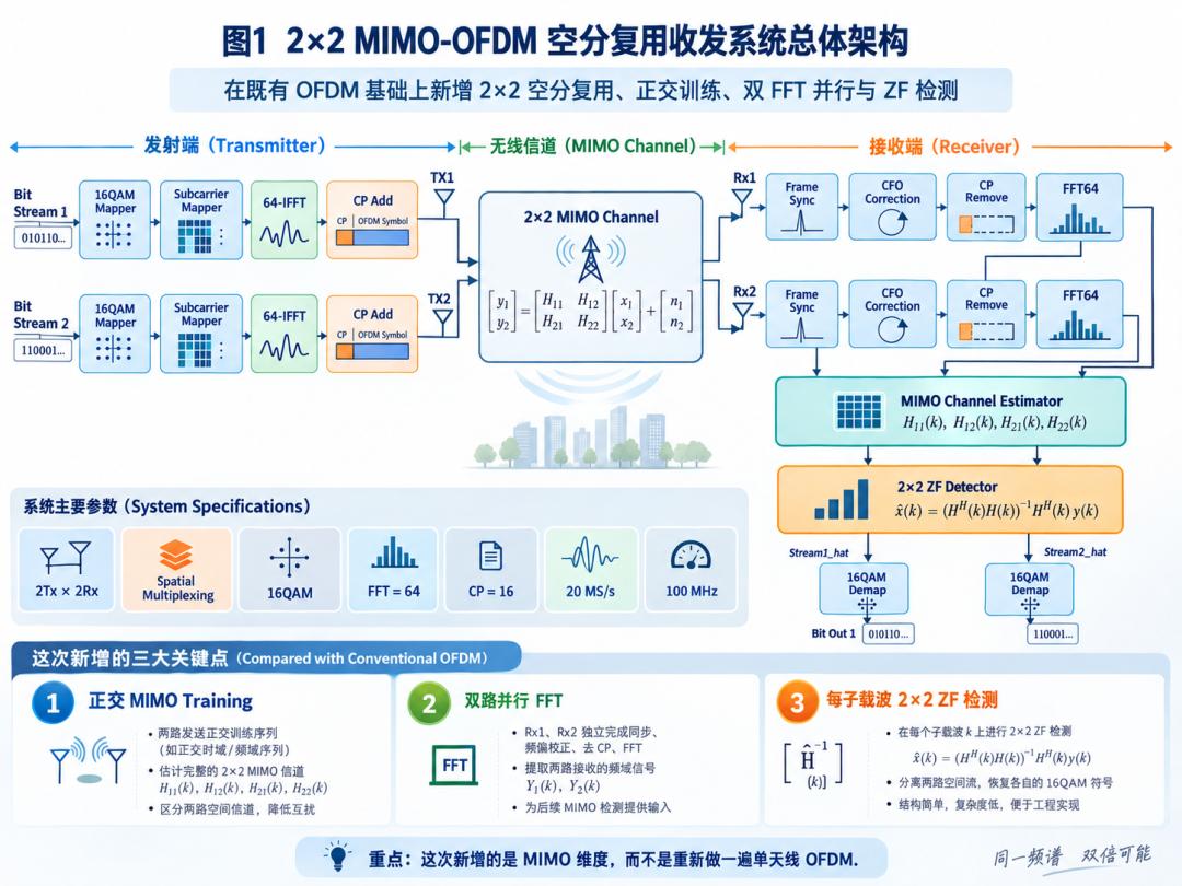
When I built the OFDM receiver earlier, the Schmidl-Cox synchronization, CFO estimation and correction, 64-point FFT, pilot-based channel estimation, equalization and 16QAM demodulation were all already working. Once you reach that point, continuing to circle around single-antenna OFDM mostly means optimizing individual modules. So this time I took a bigger step: extending the SISO-OFDM into a 2Tx × 2Rx MIMO-OFDM system, and not Alamouti — real spatial multiplexing, meaning two different data streams go out at the same moment. Two transmit antennas send two independent 16QAM spatial streams, the two receive antennas capture the superposition of those streams after they pass through different radio channels, and the FPGA pulls them apart again. What is genuinely new here is not “OFDM, duplicated.” It is three things: 2×2 channel matrix estimation, dual-path parallel reception, and 2×2 MIMO detection.
System Configuration
The whole system is fixed to this parameter set: 2Tx × 2Rx, spatial multiplexing, 16QAM, FFT = 64, CP = 16, 20 MS/s sample rate, and a 100MHz FPGA clock. The receiver uses two parallel FFTs. The transmitter carries two independent bit streams.
Stream1 → 16QAM → OFDM TX1
Stream2 → 16QAM → OFDM TX2
Both spatial streams enter the 2×2 MIMO channel together. For any given subcarrier k, the received relationship is:
y1 = H11·x1 + H12·x2 + n1
y2 = H21·x1 + H22·x2 + n2
The critical part is H11, H12, H21 and H22. Single-antenna OFDM only ever needed to estimate one H(k). In 2×2 MIMO, a subcarrier no longer corresponds to one complex channel coefficient — it corresponds to a complete 2×2 complex matrix.
Estimating Four Channels from Two Mixed Streams
This is the first real MIMO problem. If Tx1 and Tx2 transmit training sequences simultaneously, then Rx1 and Rx2 each receive a superposition of both. More elaborate orthogonal training sequences are possible, but for a first version I kept it simple and used two MIMO training symbols.
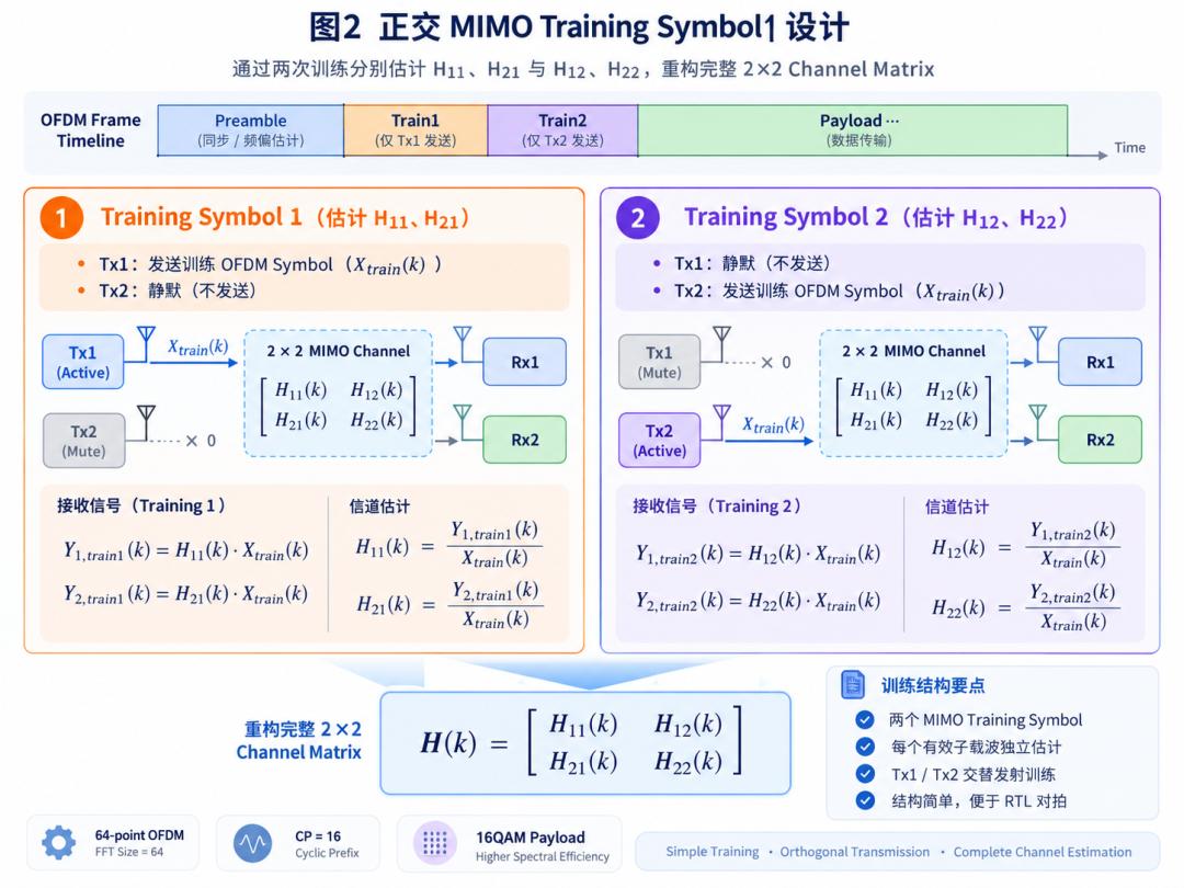
In the first training symbol, Tx1 sends a known training OFDM symbol and Tx2 stays silent. That gives:
Y1_train1 = H11 × Xtrain
Y2_train1 = H21 × Xtrain
So directly:
H11 = Y1_train1 / Xtrain
H21 = Y2_train1 / Xtrain
The second training symbol flips the roles: Tx1 silent, Tx2 transmitting. Then:
H12 = Y1_train2 / Xtrain
H22 = Y2_train2 / Xtrain
After the two training symbols, the full channel matrix on a subcarrier is available:
H(k) =
H11(k)   H12(k)
H21(k)   H22(k)
The advantages are obvious. The structure is simple, debugging is simple, and — more importantly — it is exceptionally well suited to bit-exact comparison between a Python reference model and the RTL.
Inside the FPGA: A Bank of 2×2 Matrices, Not One H
In RTL, the data organization of the channel estimation block differs completely from the single-antenna version. Both FFT outputs feed the MIMO channel estimator at the same time.
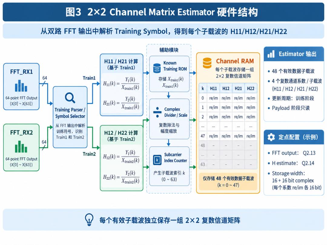
The training parser first decides whether the current symbol is Train1 or Train2. Train1 produces H11(k) and H21(k); Train2 produces H12(k) and H22(k). The training symbol itself is known, so a known-training ROM sits directly in the FPGA. After complex division and fixed-point scaling of the FFT output, the corresponding channel estimates fall out. Every valid data subcarrier stores one group: H11_re/H11_im, H12_re/H12_im, H21_re/H21_im and H22_re/H22_im.
In other words, one subcarrier maps to one complete 2×2 complex channel matrix. The training phase writes to RAM; the payload phase is essentially read-only. That keeps the MIMO detector from repeating channel estimation work.
The Hard Part: Separating Two Spatial Streams
The receiver already knows y = Hx + n. Ignoring noise for the moment, the most direct idea is x = H⁻¹y. So the first version implements a zero-forcing detector.
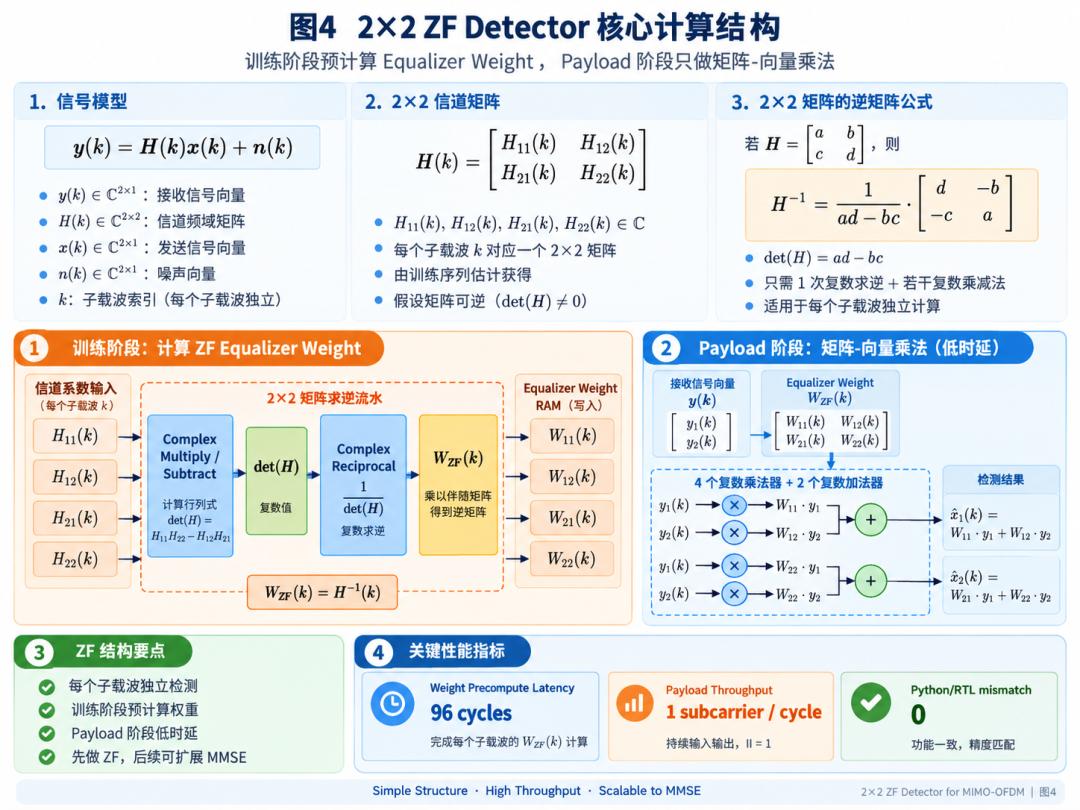
For H = [[a, b], [c, d]], the inverse is:
H⁻¹ = 1 / (ad - bc) ×
d   -b
-c   a
The formula does not look complicated, but putting it into an FPGA involves a surprising amount: complex multiplication, complex subtraction, det(H), complex reciprocal, the adjugate matrix, and complex matrix multiplication. If all of that were recomputed for every payload subcarrier, the hardware would be both complex and hard to pipeline for latency.
Matrix Inversion Moves Out of the Payload Path
H is already known from the training phase, so the corresponding equalizer weights can be computed in advance at the same time: W11(k), W12(k), W21(k) and W22(k), written into an equalizer weight RAM. Once the payload arrives, the detector only needs:
x1_hat = W11·y1 + W12·y2
x2_hat = W21·y1 + W22·y2
That is 4 complex multiplies and 2 complex adds. The entire payload detector becomes a stable streaming structure. The current design sustains 1 subcarrier per cycle, the training-phase weight precomputation takes about 96 cycles, and the Python versus RTL detection result shows mismatch = 0. This is the part I am happiest with: the complex matrix inverse moved into training, so the actual payload datapath stays clean.
Why Two FFTs and Not One
From an algorithmic standpoint, a single FFT IP could obviously be reused — run Rx1, then run Rx2. But work out the real-time budget and it stops being comfortable.
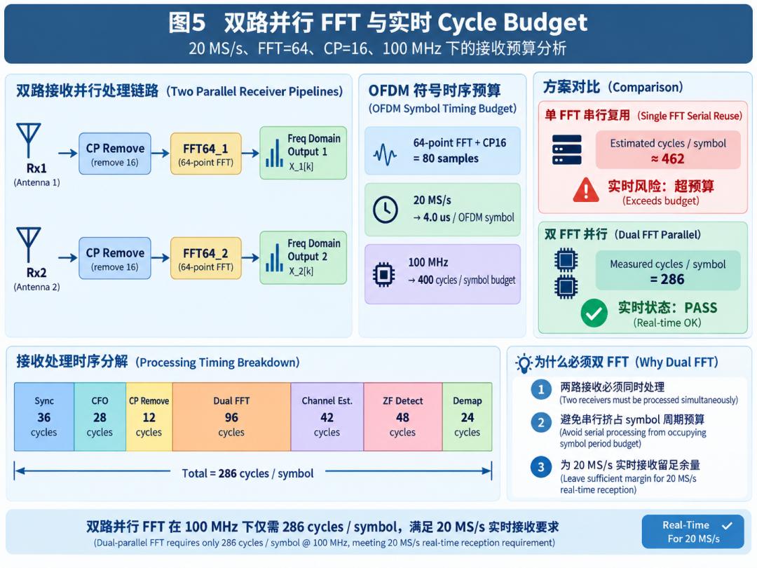
With FFT = 64 and CP = 16, a complete OFDM symbol is 80 samples. At 20 MS/s, one OFDM symbol takes 80 / 20M = 4µs. The FPGA runs at 100MHz, so 4µs is 400 cycles. Between one symbol and the next, the entire receive chain has a budget of 400 clock cycles. A single FFT serialized across two paths was estimated at about 462 cycles per symbol — already over budget. So the final structure uses two instances, FFT64_1 and FFT64_2, in parallel.
Cycle Budget with Dual FFT
| Stage | Cycles |
|---|---|
| Sync | 36 |
| CFO | 28 |
| CP removal | 12 |
| Dual FFT | 96 |
| Channel estimation | 42 |
| ZF detect | 48 |
| Demap | 24 |
| Total | 286 |
| Budget per OFDM symbol | 400 |
| Margin | 114 |
Against a 400-cycle budget, 286 cycles leaves 114 cycles of margin. Only at that point does 20 MS/s genuinely have engineering headroom.
Constellations Before and After ZF
MIMO systems are especially good to look at through constellations, because the difference before and after ZF is so obvious.
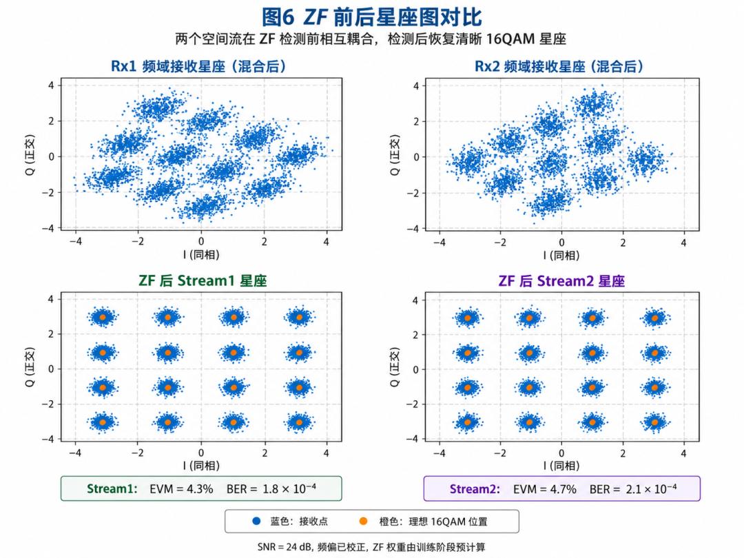
Rx1 and Rx2 show the frequency-domain signal each receive antenna sees directly after its FFT. At that stage the two spatial streams are mixed together, so it does not look like a normal 16QAM constellation at all. After the 2×2 ZF detector, Stream1 and Stream2 are separated, and the two constellations below regroup into clean 16QAM with 16 distinct points.
Under the current 24dB SNR test condition, Stream1 measures EVM = 4.3% and BER = 1.8 × 10⁻⁴, while Stream2 measures EVM = 4.7% and BER = 2.1 × 10⁻⁴. At that point it becomes visually obvious what the MIMO detector does: it pulls two already-intermingled spatial streams back out of two received signals.
ZF’s Weakness: The Channel Matrix Must Behave
At this stage I also measured a specific metric: the channel condition number. ZF is fundamentally a matrix inverse, so a high condition number means the matrix is close to ill-conditioned and H⁻¹ will amplify noise along with the signal.
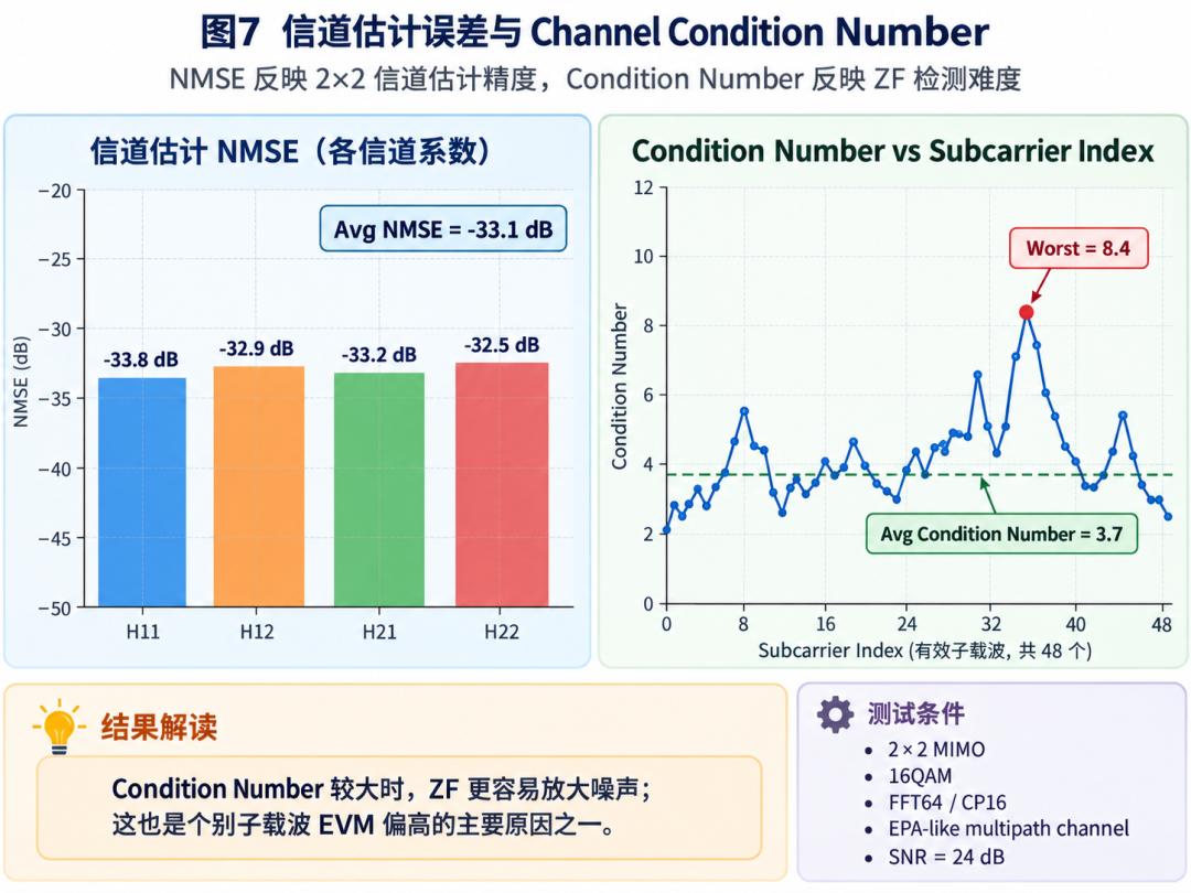
The NMSE of the four channel coefficients currently sits at H11 = −33.8 dB, H12 = −32.9 dB, H21 = −33.2 dB and H22 = −32.5 dB, averaging about −33.1 dB. Across the 48 valid subcarriers the mean condition number is about 3.7, with the worst subcarrier at roughly 8.4. That matches the post-ZF constellations: subcarriers with a high condition number tend to show larger EVM. This is exactly the natural entry point for an MMSE detector later on — ZF forces interference to zero, while MMSE trades interference rejection against noise amplification.
Python Is Not Enough: RTL Must Match
Once again I did not treat “the Python simulation looks good” as the end of the project. The entire MIMO chain was built with both a Python reference and quantized RTL running against each other.
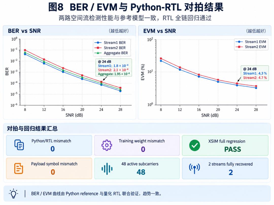
As SNR rises from 8dB to 28dB, BER on both streams falls continuously. At 24dB, Stream1 BER is 1.8 × 10⁻⁴, Stream2 is 2.1 × 10⁻⁴, and the aggregate is 1.95 × 10⁻⁴, with EVM of 4.3% and 4.7% respectively. Beyond the performance numbers, what I care about more are these results:
- Python / RTL mismatch = 0
- Training weight mismatch = 0
- Payload symbol mismatch = 0
- All 48 valid subcarriers participate in detection
- Both spatial streams recover completely
- XSIM full regression: PASS
That is how you confirm it is not just a floating-point model that appears to work, but quantized RTL that genuinely closes.
FPGA Implementation Results
The whole system was synthesized, implemented and timing-checked on FPGA.

| Metric | Result |
|---|---|
| LUT | 14.6k |
| Flip-flops | 19.8k |
| DSP | 72 |
| BRAM | 22 |
| WNS at 100MHz | +3.18 ns |
| TNS | 0.000 ns |
| Timing | PASS |
On real-time performance: 286 cycles per OFDM symbol against a 400-cycle budget, a margin of 114 cycles, zero sample drops, zero Python/RTL mismatch and a passing XSIM regression. The chain sustains continuous symbol-rate processing at 20 MS/s.
What Actually Changed from SISO to MIMO
After building this, my sense of MIMO changed. I used to think the core of it was “more antennas.” Once you actually implement it on FPGA, you realize antennas are the most superficial part of the change. What really grows is the dimensionality of the data. A subcarrier used to hold X(k), Y(k) and H(k). Now a subcarrier holds two transmit symbols, two receive symbols, four channel coefficients, one 2×2 matrix, and one 2×2 detector on top — all of which must still be processed continuously within a 4µs OFDM symbol.
So the biggest change in going from SISO to MIMO is not duplicating a few modules. It is that the system starts to genuinely contain matrices.
Compressed into three sentences: first, two orthogonal training symbols produce a complete 2×2 channel matrix per subcarrier. Second, precomputing ZF weights during training reduces the payload detector to a high-speed matrix-vector multiply. Third, dual parallel FFT keeps the entire receive chain at 286 cycles per symbol, satisfying the 20 MS/s real-time budget. Together those three turn single-antenna OFDM into a true 2×2 MIMO-OFDM spatial multiplexing receiver — and from that point, an FPGA communication system moves from single-link digital signal processing into matrix computation and spatial signal processing.
FAQ
Why use two training symbols instead of orthogonal sequences?
Because silence is the simplest orthogonal code. In the first symbol only Tx1 transmits, so Rx1 and Rx2 see H11 and H21 directly. In the second only Tx2 transmits, giving H12 and H22. Two symbols recover the full matrix with no sequence design and trivial debugging.
Why precompute the ZF weights during training?
Zero-forcing needs a matrix inverse per subcarrier, which is expensive in hardware. Since H is already known after training, the weights can be computed once and stored, leaving the payload path with just 4 complex multiplies and 2 complex adds per subcarrier at one subcarrier per cycle.
Why are two FFT instances required at 20 MS/s?
With FFT=64 and CP=16 a symbol is 80 samples, which at 20 MS/s is 4µs, or 400 cycles at 100MHz. A single FFT serialized across two receive paths was estimated at about 462 cycles, over budget, so the design uses two parallel FFT64 instances.
What limits zero-forcing performance?
The channel condition number. ZF inverts the channel matrix, so when H is near ill-conditioned the inverse amplifies noise as well as signal. Here the mean condition number is 3.7 with a worst subcarrier around 8.4, and high-condition subcarriers show larger EVM.
How do you know the RTL is actually correct?
By co-simulating a Python reference against the quantized RTL. Both training weight and payload symbol mismatches are zero across all 48 valid subcarriers, both streams recover completely, and the full XSIM regression passes.
About Aomway
Aomway has spent more than 15 years building video transmission, antenna and flight hardware for FPV and industrial UAV teams, where link robustness under interference is the deciding factor. Explore Aomway video transmitters, antennas and optical fiber systems for long-range missions in contested spectrum.
Have questions about this article? Feel free to contact us at [email protected] — we’re happy to help!