
Key Takeaways
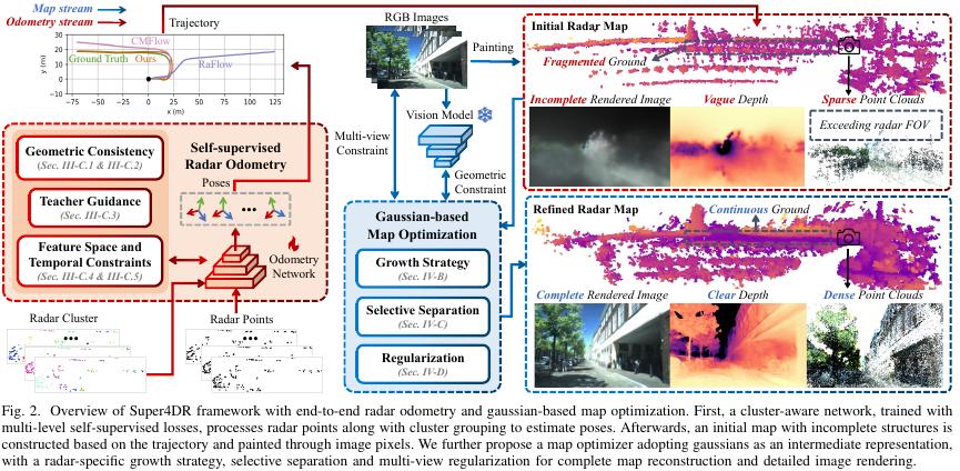
- Super4DR estimates frame-to-frame pose from sparse 4D radar point clouds, then uses camera images and a Gaussian representation to refine a map that radar alone cannot fill in.
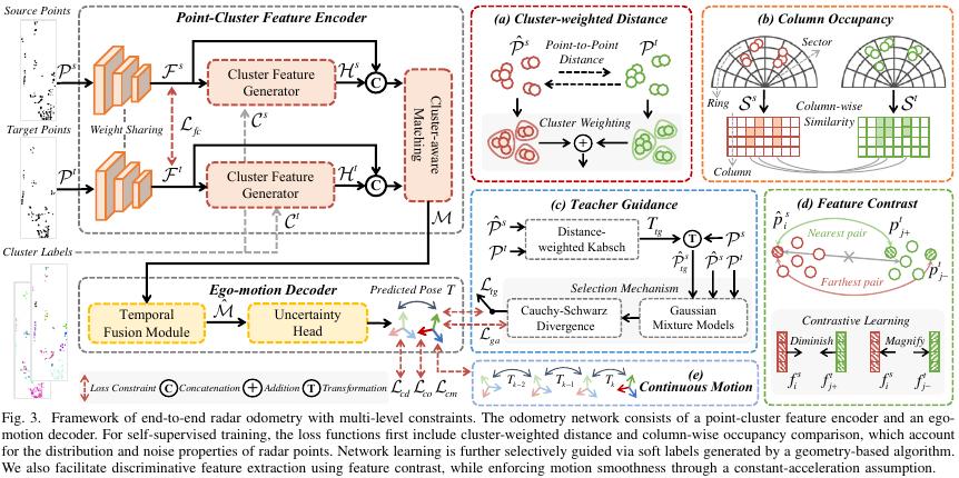
- Odometry accuracy comes from clustering: DBSCAN groups neighbouring points, a cluster-aware encoder shares geometry and features across each cluster, and a GRU-based decoder weights points before regressing rotation and translation.
- Training needs no ground-truth poses. Four self-supervised terms — cluster-weighted point distance, column occupancy, teacher-guided refinement and feature contrast — plus a constant-acceleration motion prior supply the supervision.
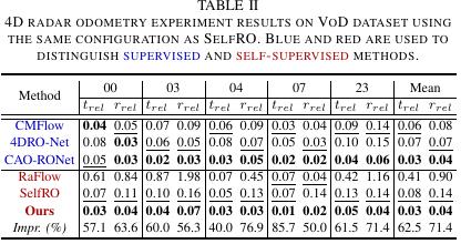
- On the VoD split used by SelfRO, mean relative translation error drops from 0.08 to 0.03 m/m and rotation error from 0.14 to 0.04°/m, a 62.5% and 71.4% relative reduction on the rounded table values.
- The method assumes a true 4D radar with elevation. A conventional automotive radar that outputs only azimuth, range and Doppler cannot use the 3D clustering and Gaussian initialization directly.
In one line: a millimeter-wave radar still sees roadside reflections at night, but when a frame holds only a few hundred points, stitching a trajectory out of them gets hard — a point near a signpost lands left in this frame and drifts in the next, so do the two blobs still correspond? Super4DR splits the problem in two: radar odometry estimates motion first, then the accumulated point cloud is converted into a Gaussian map and completed with camera images. Aomway walks through the architecture, the four self-supervised constraints and, just as importantly, how to read the reported numbers without overclaiming.
Why a Few Hundred Points Can Still Localize a Vehicle
The core difficulty is sparsity. VoD provides roughly 300–500 radar points per frame, and those points are noisy in range and angle. Matching them point-to-point between frames is unreliable, because a single reflection can shift by more than the spacing between points.
The paper’s answer is to stop matching points and start matching structure. Instead of asking whether point A in frame k corresponds to point B in frame k+1, it asks whether the cluster around A corresponds to the cluster around B. Clusters are far more stable than individual returns, which is what makes a few hundred points enough to constrain six degrees of freedom.
From Single Points to Clusters
The network input is each radar point’s 3D coordinates plus its relative radial velocity and radar cross section (RCS). The pipeline is:
- Cluster. DBSCAN groups neighbouring points, then the clusters are sampled down to a uniform point count.
- Encode. The network extracts per-point features and also aggregates the geometry and features of each cluster, then distributes the cluster feature back to the points inside it.
- Decode. The ego-motion decoder uses a GRU to combine historical motion features, assigns a weight to each point, and estimates rotation and translation.
For VoD and the authors’ own dataset, DBSCAN is set to a search radius of 3 m with a minimum of 3 points per cluster; the NTU4DRadLM setting differs.
A worked cluster example
Take three points in one cluster with lateral coordinates 2.0, 2.3 and 2.6 m. Their centre is (2.0 + 2.3 + 2.6) ÷ 3 = 2.3 m. If their three one-dimensional features are hypothetically 0.2, 0.5 and 0.8, the average is 0.5.
The real implementation concatenates the cluster centre with the multi-dimensional average feature and runs a convolution to produce the cluster feature — it does not treat 2.3 and 0.5 as a pose. The point of the example is only to show what “cluster-level aggregation” means numerically.
One caveat the authors are careful about: cluster labels reflect proximity clustering, so a cluster is not guaranteed to be one complete vehicle. A single car can split into several clusters, and two adjacent cars can merge into one.
What Supervises Training Without Ground-Truth Poses
After predicting a pose, the network transforms the previous frame’s points into the current frame and checks whether the two frames align. No human-labelled poses are used — but that does not mean there are no constraints. There are four, plus a motion prior.
1. Cluster-weighted point-to-point distance
The paper excludes low-density outliers and multiplies each cluster’s mean distance by that cluster’s share of the point count. Algebraically, if every point belongs to a counted cluster, the sum of (cluster mean × point share) equals the mean distance over all points. Large clusters contribute more because they contain more points — not because each point in a large cluster earns extra weight. That distinction matters when you try to reproduce the loss.
Example: cluster A has 8 points with mean distance loss 0.1; cluster B has 2 points with mean 0.4. The result is 8/10 × 0.1 + 2/10 × 0.4 = 0.16. If you instead averaged the two cluster means with equal weight, you would get 0.25. When cluster assignment or outlier handling changes, the actual computation has to be checked against the implementation.
2. Column occupancy
Points are discretized into a polar grid by radial distance and azimuth, and occupancy vectors are compared column by column. If one azimuth column reads [1,1,0] in one frame and [1,0,0] in the other, the cosine similarity is 1/√2 ≈ 0.707, so the corresponding difference is about 0.293.
This term is robust to small motion inside a cell — occupancy does not change until a point crosses a cell boundary, at which point the result can flip. The paper excludes empty columns, because a zero vector cannot be normalized.
3. Teacher guidance
A geometric teacher takes the network prediction as an initial value and refines it with distance-weighted Kabsch. The authors represent the point cloud as a Gaussian mixture model and compare the Cauchy–Schwarz divergence before and after refinement. Only if the divergence decreases is the refined pose adopted as a soft label; if it fails the check, the divergence between the two frames’ Gaussian mixtures continues to provide the constraint instead.
4. Feature contrast, plus a motion prior
A feature contrastive term helps separate matched from unmatched points, and a continuous-motion constraint assumes constant acceleration. That last assumption is worth flagging: a sudden hard brake or a sharp turn on the road is exactly where a constant-acceleration prior is least applicable, and the paper does not claim otherwise.
How Images Fill In the Radar Map
Stacking multiple radar frames produces a map that may still be sparse, missing the ground, and blind to everything outside the radar field of view — even when the trajectory is accurate. So the paper accumulates points along the trajectory, builds a Gaussian representation together with the aligned images, and constrains the map with a differentiable render plus geometric priors from a visual foundation model.
Think of each Gaussian as a spatial ellipsoid with a centre, scale and orientation. Map optimization keeps adjusting them to reduce the difference between the rendered image and the observation. A single pixel’s colour cannot uniquely determine its 3D position, which is why the paper leans on multi-view overlap for geometric consistency.
A worked compositing example
Along one line of sight, suppose the front and rear Gaussians sit at depths of 10 m and 12 m with opacities of 0.6 and 0.5 for that pixel. Under the paper’s forward compositing formula, the front contributes 0.6 × 10 = 6, and the rear contributes after the residual transmittance: (1 − 0.6) × 0.5 × 12 = 2.4. The composited depth term is 8.4 m.
Note that 0.2 of transmittance remains, so 8.4 is the unnormalized accumulated value of that formula — it is not a normalized average of the two depths. Change either depth or either opacity and the render changes, which is precisely the signal used to adjust the Gaussians.
Radar-specific tricks for sparse data
- Visual depth priors supply the missing ground plane.
- Local geometry-driven splitting and interpolation of Gaussians fill structural gaps.
- Selective separation handles sky-related Gaussians, combined with neighbourhood pruning to cut floaters.
One honest limitation: structure recovered inside the camera’s field of view is influenced by the visual prior. It should not be treated as radar-measured returns.
Reading the Numbers
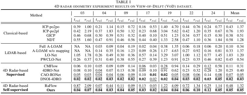
VoD provides roughly 300–500 radar points per frame. The paper evaluates relative pose error over trajectory segments from 20 m to 160 m in 20 m bins; translation is reported in m/m and rotation in °/m. On the same five-sequence VoD split used by SelfRO, Table II reports:
| Method | Mean relative translation trel (m/m) ↓ | Mean relative rotation rrel (°/m) ↓ |
|---|---|---|
| SelfRO | 0.08 | 0.14 |
| Super4DR | 0.03 | 0.04 |
From the table values, relative translation error falls by (0.08 − 0.03) ÷ 0.08 = 62.5% and rotation error by about 71.4%. These percentages are computed from the rounded means printed in the table, so the unrounded values may differ slightly.
Two cautions. First, these are different error terms — neither one alone should be described as the improvement of the whole system. Second, the authors adopt SelfRO’s sequence split (noting that SelfRO was not open-sourced at the time), and Table I uses a different set of sequences. The means from the two tables must not be mixed.
Map results: watch which poses were used
The mapping experiment has to be read separately, because the paper builds initial maps on five VoD sequences twice — once with ground-truth poses and once with its own odometry. The ground-truth run isolates the effect of map optimization.
With ground-truth poses, the paper reports a mean F-score of 0.513 for Super4DR versus 0.344 for 3DGS, evaluated against a LiDAR map with a 0.3 m distance threshold. F-score measures how well reconstructed points match the reference — it is not a measure of visual image quality.
In the same per-sequence table, the five runs using the method’s own odometry score 0.394, 0.438, 0.389, 0.433 and 0.402, an arithmetic mean of about 0.411. Comparing that with 0.513 shows how much pose error still costs the map.
The authors also try thermal imaging to assist map optimization, for example on the NTU4DRadLM Garden sequence. Because the visual model used does not support normal estimation on thermal images, that run omits the normal constraint.
Runtime
The paper reports about 15.9 ms for odometry. That is the measurement scope for that component only; map optimization, image acquisition and full-system latency must be counted separately. Optimizing the map also needs synchronized, calibrated cameras and decent image quality. The authors acknowledge that accumulated odometry drift still affects the map, and list loop closure and pose-graph optimization as future work.
Before You Port This to Your Own Sensor
Radar points are few, so cluster structure, temporal continuity and image information each contribute a different constraint. Bringing this to your own platform, the first thing to confirm is whether the output actually includes elevation, height, RCS and raw detections — and then whether the camera can be calibrated reliably.
A conventional automotive radar without elevation or height cannot reuse the paper’s 3D clustering and Gaussian initialization directly. In that case the more transferable ideas are the 2D occupancy formulation and the frame-to-frame consistency logic, not the full 3D pipeline.
Have questions about this article? Feel free to contact us at [email protected] — we’re happy to help!
Frequently Asked Questions
What makes 4D radar different from ordinary automotive radar here?
It provides elevation, so points form a true 3D cloud with height. That enables 3D DBSCAN clustering and 3D Gaussian initialization. A radar reporting only azimuth, range and velocity lacks the vertical dimension, and the method’s 3D steps cannot be applied as written.
Why is clustering necessary instead of matching points directly?
Because at 300–500 points per frame, a single reflection can shift further than the spacing between points, making point-to-point correspondence unreliable. Cluster-level features are far more stable, so the network matches structures rather than individual returns and weights points before regressing pose.
Does the method need ground-truth poses for training?
No. Supervision comes from cluster-weighted point distance, column occupancy, teacher-guided Kabsch refinement gated by Cauchy–Schwarz divergence, and feature contrast, plus a constant-acceleration motion prior. The paper trains end to end without labelled trajectories.
What do the 0.03 and 0.04 errors actually mean?
They are mean relative errors over 20–160 m trajectory segments: 0.03 m/m translation and 0.04°/m rotation on the SelfRO VoD split. Against SelfRO’s 0.08 and 0.14, that is a 62.5% and 71.4% reduction computed from the rounded table values.
Can the map be trusted where the camera sees?
Partly. Structure recovered inside the camera’s field of view is shaped by the visual depth prior, so it is not radar-measured data. F-score against a LiDAR reference is the honest metric here, and it drops from 0.513 with ground-truth poses to about 0.411 with the method’s own odometry.
References
Li et al., Super4DR: 4D Radar-centric Self-supervised Odometry and Gaussian-based Map Optimization, IEEE Transactions on Robotics, 2026, arXiv v2.
Paper: arxiv.org/html/2512.09608v2
Project: github.com/NEU-REAL/Super4DR
This article is a study and technical-exchange summary. Specific conclusions should be checked against the paper and the actual experimental conditions. Original Chinese article: mp.weixin.qq.com.
About Aomway
Aomway designs and manufactures FPV video transmitters, antennas, cameras and goggle systems for drone pilots worldwide, with more than fifteen years in the UAV industry. Its hardware serves racing, long-range and professional aerial platforms where low-latency video and reliable RF links matter most.