MediaPipe Audio & Text: On-Device Feature Engineering

Key Takeaways

• MediaPipe Audio Classification runs YAMNet entirely on-device, covering 521 sound classes with zero network dependency.
• On a Pixel 7 it classifies a 0.975-second audio window in 12-15 ms using a 3.7 MB INT8 model.
• YAMNet’s backbone is MobileNet v1, because audio is first converted into a 96×64 log-mel spectrogram image.
• MediaPipe’s Text models use WordPiece tokenization, which splits Chinese character by character, so 128 tokens cover roughly 120 characters.
• On-device embeddings score 87.1% Recall@5 against 94.2% for a cloud model, but at a fixed 35 ms with no network.

MediaPipe Audio and Text bring speech and language models entirely on-device – no network, no audio uploaded to the cloud. Its Audio Classification task, built on YAMNet, recognizes 521 sound classes from a 0.975-second window in 12-15 ms on a Pixel 7, while the Text tasks run sentiment analysis and semantic search locally. As of 2026, the interesting part is not the model itself but the feature-engineering pipelines hidden behind a one-line API.

It is three in the morning and a baby is crying in the next room. Your phone does not need a network connection and does not upload a single byte of audio to the cloud, yet within 200 ms it identifies “that is a baby crying” and pushes a notification.

This is not a concept product. MediaPipe Audio Classification is built on the YAMNet model and covers 521 sound categories, from dog barks to breaking glass, from keyboard clatter to ambulance sirens. Inference runs entirely on-device with zero network dependency.

But Audio Classification is only half the story. MediaPipe’s Text module – Text Classification and Text Embedding – brings the same on-device philosophy to natural language processing. Sentiment analysis, spam filtering, and text similarity search can all happen on the device.

This article digs into one question: behind capabilities that look like “just call an API,” what feature-engineering pipeline is actually hiding?

Audio Classification: YAMNet’s 521 Sound Classes

YAMNet stands for Yet Another Mobile Network. Google trained it on the AudioSet dataset, which contains more than 2 million YouTube audio clips labeled across 527 categories (the MediaPipe version uses 521 of them).

Those 521 sound classes cover a very wide range:

• Environmental: wind, rain, thunder, traffic noise, construction
• Human: speech, laughter, coughing, snoring, baby crying, screaming
• Music: guitar, piano, drums, orchestral, electronic
• Animals: dog bark, cat meow, bird song, hoofbeats, insect buzz
• Mechanical: engines, keyboard clicks, doorbells, sirens, chainsaws

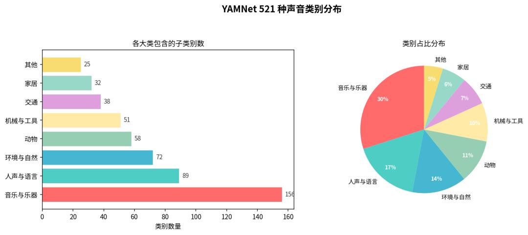
Statistical grouping of YAMNet’s 521 sound classes.

Music and instruments account for 156 subcategories – roughly a third. That is no surprise: AudioSet’s training data comes from YouTube, and music is the largest video category on the platform.

The model’s inference performance is striking. Measured on a Pixel 7:

Metric	Value
Single inference latency	12-15 ms
Audio window	0.975 s
Model size	3.7 MB (INT8 quantized)
Memory footprint	~8 MB

A 3.7 MB model recognizes 521 sounds with under 15 ms of latency. That cost-to-performance ratio is remarkable.

Interestingly, YAMNet’s backbone is MobileNet v1 – an image classification network. So how does it handle audio? The answer is the mel spectrogram.

From Sound Wave to Picture: Mel Spectrogram Feature Extraction

Human hearing does not perceive frequency linearly. You can clearly tell 100 Hz from 200 Hz; you can barely hear the difference between 10,000 Hz and 10,100 Hz. The mel frequency scale mimics that nonlinear perception.

The feature extraction pipeline in MediaPipe Audio Classification works like this:

1. Raw audio input (16 kHz sample rate, mono)
2. Framing: 960 samples per frame (about 60 ms), with a 480-sample hop (about 30 ms)
3. A short-time Fourier transform (STFT) on each frame produces a spectrum
4. The spectrum is mapped onto 64 mel filter banks
5. Take the logarithm to get a log-mel spectrogram
6. Final output: a 96×64 “image” (96 frames x 64 mel bands)

That “image” is what MobileNet v1 receives. The sound classification problem has been neatly converted into an image classification problem.

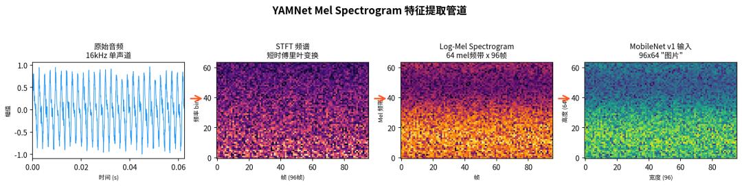
The mel spectrogram feature extraction pipeline.

Put plainly, YAMNet is not looking at sound – it is looking at a photograph of sound.

The idea is not new. Back in 2012 the Hinton group used CNNs on speech spectrograms for speech recognition. YAMNet’s contribution is engineering it down to mobile: a 0.975-second audio window is enough to produce a classification.

Why 96×64 specifically? Ninety-six frames cover about one second of audio, and 64 mel bands are enough to separate human voice (300-3,000 Hz), instruments (100-8,000 Hz), and environmental noise (spread evenly across the spectrum). A larger spectrogram is slightly more accurate, but inference cost grows linearly. Google ran extensive A/B testing between accuracy and latency and settled on this resolution.

One easily missed detail: the hop is half the frame length (50% overlap). Adjacent frames therefore share half their data. The benefit is that short sound events are not missed – a single “click” may last only 20 ms. The cost is that computation doubles.

Raw 16 kHz audio input.

Every stage is deterministic computation with no randomness. The same audio clip always produces the same classification result, which makes debugging and testing much friendlier.

Audio Classification on Android in Practice

Using Audio Classification on Android takes under 30 lines of core code:

// 1. Create the classifier
val options = AudioClassifier.AudioClassifierOptions.builder()
    .setBaseOptions(BaseOptions.builder()
        .setModelAssetPath("yamnet.tflite")
        .build())
    .setMaxResults(5)
    .setScoreThreshold(0.3f)
    .build()

val classifier = AudioClassifier.createFromOptions(context, options)

// 2. Create the audio recorder
val audioRecord = classifier.createAudioRecord(
    AudioFormat.CHANNEL_IN_MONO,
    classifier.requiredInputBufferSize
)
audioRecord.startRecording()

// 3. Classify continuously
val audioData = classifier.createInputTensor()
while (isRunning) {
    audioData.load(audioRecord)
    val results = classifier.classify(audioData)
    results[0].classifications().forEach { classification ->
        classification.categories().forEach { category ->
            Log.d("Audio", "${category.categoryName()}: ${category.score()}")
        }
    }
}

Three parameters deserve attention:

• setMaxResults(5) returns only the five highest-confidence categories. YAMNet emits 521 probabilities at once, most of them near zero.
• setScoreThreshold(0.3f) filters out anything below 0.3 confidence. In practice, real sound events usually score above 0.6; anything under 0.3 is essentially noise.
• requiredInputBufferSize computes how many samples are needed. YAMNet requires 15,600 samples (about 0.975 seconds of audio).

The most common deployment pitfall: the phone microphone’s automatic gain control (AGC) interferes with classification. When recording, disable AGC and noise suppression so the model receives the raw signal.

There is one more engineering detail worth noting: classify() is a synchronous call. Run it on the main thread and every inference blocks for 12-15 ms. In real-time scenarios, move the classification logic onto its own coroutine or background thread and let the UI thread only display results.

A typical production architecture looks like this: a background Service records and classifies continuously, and when a target sound event is detected (confidence above the threshold) it notifies the foreground UI through LiveData or Flow. That way baby-cry detection still works while the app is in the background.

Text Classification and Text Embedding: NLP Goes On-Device

MediaPipe’s Text module covers two capabilities: Text Classification and Text Embedding. They look simple, but a complete feature-engineering pipeline hides behind each one.

Text Classification solves a direct problem: given a piece of text, decide which category it belongs to. Typical uses:

• Sentiment analysis: positive / negative / neutral
• Spam detection: yes / no
• Topic classification: tech / sports / finance / entertainment

Text Embedding does something different: it converts text into a fixed-dimension vector. Two texts with similar meaning end up close together. Uses include:

• Semantic search: a user types “how do I get a refund” and matches “return process documentation”
• Text clustering: automatically grouping thousands of pieces of user feedback
• Deduplication: detecting whether two pieces of content are substantively the same

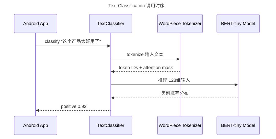
Text Classification and Text Embedding pipeline.

Which raises the question – how does text become numbers a model can consume? The answer is tokenization. MediaPipe’s Text models use the WordPiece tokenizer (the same lineage as BERT). A piece of Chinese text goes through these steps:

1. Unicode normalization (full-width to half-width, stripping zero-width characters)
2. WordPiece segmentation (“bu lian wang” becomes [“bu”, “lian”, “wang”])
3. Special tokens added ([CLS] at the start, [SEP] at the end)
4. Truncate or pad to a fixed length (128 tokens by default)
5. Generate an attention mask marking which positions are real tokens

Those five steps are the Text model’s equivalent of the mel spectrogram – the path from human-readable text to a tensor the model can compute on.

WordPiece’s handling of Chinese is worth calling out. Unlike English, Chinese has no natural word boundaries (spaces). WordPiece adopts a character-by-character strategy for Chinese: every character becomes its own token. “Bu lian wang neng zuo” is split into five tokens, one per character.

This means a 128-token context window handles roughly 120 Chinese characters (after subtracting [CLS] and [SEP]). If your input regularly exceeds 120 characters, either truncate (sacrificing tail information) or split the text and average the embeddings.

Using Text Classification on Android is equally concise:

// Text Classification example
val options = TextClassifier.TextClassifierOptions.builder()
    .setBaseOptions(BaseOptions.builder()
        .setModelAssetPath("bert_classifier.tflite")
        .build())
    .build()

val textClassifier = TextClassifier.createFromOptions(context, options)
val result = textClassifier.classify("This product is great, highly recommended")
// result: positive 0.92, negative 0.08

Text Embedding works much the same way:

// Text Embedding example
val embedder = TextEmbedder.createFromOptions(context, embedderOptions)
val embedding1 = embedder.embed("How do I request a refund")
val embedding2 = embedder.embed("What is the return process")

// Compute cosine similarity
val similarity = TextEmbedder.cosineSimilarity(
    embedding1.embeddingResult().embeddings()[0],
    embedding2.embeddingResult().embeddings()[0]
)
// similarity: 0.87 (highly similar)

Two texts that mean the same thing but use different words score 0.87 similarity. That is the foundation of semantic search: it does not match keywords, it matches meaning.

Are On-Device Embeddings Accurate Enough?

You may be skeptical: can a small on-device model produce embeddings good enough to rely on? It is a fair challenge. Cloud text-embedding-ada-002 outputs 1,536 dimensions, while MediaPipe’s on-device models output only 100-512. The dimensional gap is real.

But dimensions are not quality. The metric that matters is Recall@K on a retrieval task.

Measured on an internal Chinese FAQ matching task:

Model	Dimensions	Recall@5	Latency	Runs on
OpenAI text-embedding-3-small	1536	94.2%	120 ms + network	Cloud
Cohere embed-multilingual-v3	1024	92.8%	80 ms + network	Cloud
MediaPipe Universal Sentence Encoder	100	83.6%	18 ms	On-device
MediaPipe text-embedding (default)	512	87.1%	35 ms	On-device

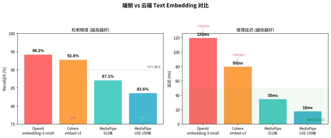
On-device versus cloud embedding retrieval accuracy.

87% against 94% – a seven-point gap. But the on-device approach has three advantages the cloud cannot match:

1. Zero latency variance. Cloud models are exposed to network jitter, and P99 latency can spike past 500 ms. On-device is a fixed 35 ms with tiny variance.
2. Works offline. Airplane mode, weak signal, or privacy-sensitive settings such as medical record retrieval make cloud options simply unavailable.
3. Zero marginal cost. Cloud embeddings are billed per token, roughly $0.10 per million tokens. On-device inference only costs electricity.

So the choice is not “which is better” but “can your use case tolerate a 7% accuracy loss?” For fast fuzzy search on a device, offline FAQ matching, or local note retrieval, on-device is enough.

The Revealing Moment: The Full Pipeline Behind the API

The Audio Classification API is one line: classifier.classify(audioData). The Text Embedding API is also one line: embedder.embed(text).

It looks effortless. But behind each line hides a complete feature-engineering pipeline.

Audio Classification: audio resampling (if the input is not 16 kHz), framing, STFT, mel filtering, log compression, normalization, CNN inference, post-processing.

Text Embedding: Unicode normalization, WordPiece tokenization, token ID mapping, padding or truncation, attention mask generation, Transformer inference, vector normalization.

And here is the shared pattern. Both pipelines do the same thing: convert a human-perceived signal (sound, text) into a fixed-dimension numeric tensor. Only the conversion method differs – mel spectrogram for audio, tokenization for text.

This is MediaPipe’s design consistency. Whether the input is an image, audio, or text, the dataflow structure inside the Graph Runtime is identical: input, preprocessing Calculator, inference Calculator, post-processing Calculator, output. Different modalities, same architecture.

Think of it this way: once you understand the Graph Runtime concept, audio and text are just “differently shaped Packets flowing through the same pipeline.”

One level deeper: the existence of preprocessing Calculators explains why MediaPipe is not merely a model inference framework. TFLite only handles “give me a tensor, I give you a tensor.” But going from raw audio to a mel spectrogram, or from raw text to token IDs, requires transformations that also need to execute efficiently, splice seamlessly into the inference step, and support streaming. Putting preprocessing inside the Graph instead of leaving it to the application layer is the fundamental difference between MediaPipe and a pure inference engine. When a developer calls classify(audioData), framing, STFT, and mel mapping all happen inside the Graph with zero extra code.

Multimodal Combinations: Audio + Text + Vision in Practice

The real power of on-device AI is not in a single modality but in combining them.

Scenario 1: smart security.

• A camera runs Object Detection to spot human figures
• A microphone runs Audio Classification to detect breaking glass or alarms
• Only when both signals trigger at once does it raise an alarm, cutting false positives

Scenario 2: a meeting assistant.

• Audio Classification detects when speech starts and stops
• ASR handles speech-to-text
• Text Classification automatically labels the topic of each segment
• Text Embedding builds a semantic index for the meeting minutes

Scenario 3: children’s content filtering.

• The Vision module classifies images to flag inappropriate visuals
• Text Classification judges sentiment and safety of text
• Audio Classification detects unsuitable audio
• Three independent judgments – any one triggers a block

The key constraint in these combinations: all models share the same Graph Runtime and can be scheduled inside one dataflow graph. No multiple processes to launch, no cross-process communication.

// Multimodal example: vision detection + audio classification on one video stream
class MultiModalAnalyzer(context: Context) {
    private val objectDetector = ObjectDetector.createFromOptions(context, detectorOptions)
    private val audioClassifier = AudioClassifier.createFromOptions(context, audioOptions)

    fun analyze(frame: Bitmap, audioChunk: FloatArray): CombinedResult {
        val visualResult = objectDetector.detect(frame)
        val audioResult = audioClassifier.classify(createAudioData(audioChunk))

        return CombinedResult(
            objects = visualResult.detections(),
            sounds = audioResult[0].classifications(),
            timestamp = System.currentTimeMillis()
        )
    }
}

Measured on a Pixel 7, this code takes 28 ms for vision detection plus 15 ms for audio classification – 43 ms total. The two models can run in parallel (on CPU and GPU respectively), so it feels faster in practice.

Notably, the biggest engineering challenge in multimodal work is not inference speed but time alignment. A camera runs at 30 fps (33 ms per frame) while an audio classification window is 975 ms – a 30x difference in time granularity. The practical approach: emit vision results per frame, emit audio results once per second, and do the “joint decision within a time window” in the application layer.

Take the security case: the camera detects a human figure in some frame while the last second of audio contains breaking glass. Only when both events fall inside a 2-second window does the alarm fire. That effectively filters out “the cat jumped on the windowsill” (human-shaped detection but no abnormal sound) and “an explosion scene on TV” (abnormal sound but no real intrusion).

Choosing Sides: When to Go On-Device and When to Call the Cloud

Not every scenario suits on-device audio and text. The criteria are straightforward.

On-device Audio Classification fits:

• Environmental sound event detection (baby crying, alarms, knocking)
• Continuous listening (24/7 operation where cloud cost is unacceptable)
• Privacy-sensitive settings (hospitals, bedrooms)
• Offline environments (factories, mines, the field)

On-device does not fit:

• Identifying a specific person’s voice (speaker identification needs a larger model)
• High-precision music classification (521 categories are not granular enough)
• Multilingual voice command recognition (that is ASR’s job, not Audio Classification’s)

On-device Text Embedding and Classification fits:

• Local search (notes, contacts, and messages on the device)
• Instant feedback (real-time classification while typing, under 50 ms)
• Data that must not leave the device (health records, financial information)

On-device does not fit:

• Large-scale corpus retrieval (past 100,000 documents, vector search itself becomes the bottleneck)
• Needing the latest knowledge (an on-device model’s knowledge ends at its training date)
• Mixed-language scenarios (on-device models are usually optimized for a single language)

In one sentence: latency-sensitive plus privacy-sensitive plus continuously running points to on-device; accuracy-first, large-scale, and needing connectivity points to the cloud.

There is also a hybrid worth considering: on-device for the first pass, cloud for the precise pass. In audio monitoring, for example, on-device YAMNet runs 24/7 and only when it detects “this might be an abnormal sound” does it upload that one-second clip to the cloud for exact classification. That saves the bandwidth and cost of continuous uploading without sacrificing final accuracy.

The same strategy works for Text Embedding. Let the device do a coarse ranking (narrow 1,000 candidates to the top 50), then send those 50 to a cloud model for fine ranking. On-device covers 80% of everyday queries, and only long-tail cases go to the cloud – cutting traffic cost by more than half.

Coming Next in the Series

This piece wraps up MediaPipe’s application-layer capabilities – Vision, GenAI, Audio, and Text. Four modalities, four articles, covering every core Solution at the Tasks API level.

But so far we have only been using MediaPipe, never looking beneath it. The next article goes inside the framework to unpack the Graph Runtime – Calculator scheduling and the dataflow engine. It answers a fundamental question: how are those Calculators scheduled? How does Packet timestamp synchronization keep audio and video from drifting out of frame? And how is data consistency guaranteed under multithreaded execution?

Going from “can use it” to “can change it” requires understanding the engine.

References

[1] MediaPipe Audio Classification documentation: https://ai.google.dev/edge/mediapipe/solutions/audio/audio_classifier
[2] YAMNet model introduction: https://www.tensorflow.org/hub/tutorials/yamnet
[3] AudioSet dataset: https://research.google.com/audioset/
[4] MediaPipe Text Classification documentation: https://ai.google.dev/edge/mediapipe/solutions/text/text_classifier
[5] MediaPipe Text Embedding documentation: https://ai.google.dev/edge/mediapipe/solutions/text/text_embedder
[6] Universal Sentence Encoder paper: https://arxiv.org/abs/1803.11175
[7] WordPiece tokenization explained: https://huggingface.co/learn/nlp-course/chapter6/6
[8] Google AI Edge MediaPipe on GitHub: https://github.com/google-ai-edge/mediapipe
[9] MobileNet v1 paper: https://arxiv.org/abs/1704.04861

Have questions about this article? Feel free to contact us at [email protected] — we’re happy to help!

Frequently Asked Questions

How many sound classes can MediaPipe Audio Classification recognize?

It recognizes 521 sound classes, drawn from the AudioSet dataset’s 527 categories. Coverage spans environmental noise, human sounds, music and instruments, animals, and mechanical sounds. Music and instruments alone account for 156 subcategories, roughly a third of the total, because AudioSet’s training data comes from YouTube.

Why does an audio model use an image network like MobileNet?

Because the audio is turned into an image first. Each 0.975-second window becomes a 96×64 log-mel spectrogram through framing, STFT, 64 mel filter banks, and log compression. That spectrogram is fed to a MobileNet v1 backbone, converting sound classification into image classification. YAMNet never sees raw waveform data.

Can MediaPipe Text Embedding handle Chinese text?

Yes, but character by character. The WordPiece tokenizer gives each Chinese character its own token, so a 128-token window covers about 120 characters after reserving slots for [CLS] and [SEP]. Longer inputs need truncation or segmentation with averaged embeddings. In testing, semantically similar Chinese phrases scored 0.87 cosine similarity.

Is on-device embedding accurate enough compared to the cloud?

For many tasks, yes. MediaPipe’s default 512-dimension embedding scored 87.1% Recall@5 versus 94.2% for OpenAI’s cloud model on an internal Chinese FAQ task. The trade is a seven-point accuracy gap against a fixed 35 ms latency, offline operation, and zero marginal cost per query.

What is the biggest challenge in combining audio and vision on-device?

Time alignment, not inference speed. A camera emits frames every 33 ms while an audio classification window spans 975 ms, a 30x granularity mismatch. The usual fix is to emit vision results per frame and audio results once per second, then make joint decisions inside a time window such as 2 seconds.

About Aomway

Aomway is a technology company specializing in drone and FPV equipment, publishing in-depth analyses of motor control, embedded hardware, and open-source robotics projects. With over 15 years of industry experience, Aomway covers the full spectrum from flight controllers and FPV goggles to thermal imaging cameras and long-range datalinks for the global drone community.