
Key Takeaways
- The script models a circular concentric-ring phased array at 10 GHz with 10 rings plus a center element at half-wavelength spacing.
- Steering the beam requires changing only two parameters, theta0 and phi0; the default points at 45 degrees in the x-z plane.
- Odd rings are offset by half an angular step, which evens out nearest-neighbor spacing and suppresses periodic grating lobes.
- The default aperture radius is 5 wavelengths, and the script runs a numerical grating-lobe check over a 301 by 301 u-v grid.
- Outputs include element coordinates, 2D and 3D patterns, a four-angle scanning demo, and a CSV of element amplitudes and phases.
This MATLAB script designs a circular planar phased array and scans its beam electronically by changing just two angles. The array is a concentric-ring grid in the x-y plane with uniform amplitude excitation and a scan phase taper, so steering toward any direction is a one-line edit to theta0 and phi0. It targets MATLAB R2016b or later and assumes isotropic elements with mutual coupling neglected.
Why a Circular Array Instead of a Rectangular Grid
A circular aperture has no edge corners. That makes the radiation pattern rotationally symmetric, with sidelobes that stay uniform as the beam rotates. For the same aperture size and gain, a circular array also saves the four corner elements a rectangular grid would need, because those corners contribute little to the main beam while adding cost and weight.
Array Geometry and Element Placement
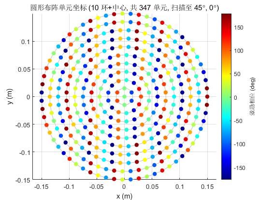
The array is a concentric-ring grid in the x-y plane with boresight along +z. A single element sits at the center, and Nring concentric rings surround it at a radius spacing of dr. The number of elements on each ring follows the arc spacing, so the circumference is divided into roughly equal steps:
Nm = round(2*pi*rm/dr)
With the default settings of 10 rings and dr = lambda/2, the script reports 347 elements and an aperture radius of 5 wavelengths. Odd-numbered rings are rotated by half an angular step when stagger is true, which improves nearest-neighbor uniformity and lowers periodic grating lobes. The script prints the minimum and maximum nearest-neighbor spacing as a self-check so you can confirm the geometry before looking at any pattern.
Default Parameters
| Parameter | Value | Meaning |
|---|---|---|
f |
10 GHz | Operating frequency |
lambda |
0.03 m | Wavelength, computed as c/f |
Nring |
10 | Concentric rings, excluding the center element |
dr |
lambda/2 | Ring radius spacing, also the nominal arc spacing |
stagger |
true | Offset odd rings by half an angular step |
theta0 |
45 deg | Scan angle measured from the +z axis |
phi0 |
0 deg | Scan angle measured from the +x axis |
Beam Scanning: Two Angles, One Phase Taper
Scanning works by applying a progressive phase across the aperture. The excitation weights are:
w = exp(-1j*k*(xe*u0 + ye*v0))
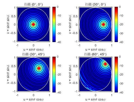
Here u0 and v0 are the pointing direction expressed in u-v space, where u = sin(theta)cos(phi) and v = sin(theta)sin(phi). Because every element shares the same amplitude and only the phase changes, the pattern shape stays constant as the beam sweeps.
To trade gain for lower sidelobes, multiply the weights by a radial amplitude taper such as w = w .* (1 - (r/R).^2).^p, where r is each element’s distance from the center and R is the aperture radius.
Grating-Lobe Check
The script evaluates the array factor on a 301 by 301 grid in u-v space and restricts it to the visible region where u^2 + v^2 <= 1. It then masks out the main lobe using a radius of twice the main-lobe half width, lambda/(2R), and takes the highest remaining level. If that level exceeds -10 dB the script warns that a grating lobe may exist; otherwise it reports a clean visible region.
Because the check works directly on the u-v grid rather than on an assumed lattice, it applies to any element layout, not only the concentric-ring geometry used here.
What the Script Produces
Four figures plus a CSV export:
- Element coordinates and ring topology, colored by excitation phase
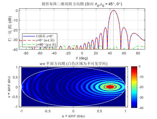
- A 2D pattern with scan-plane, phi = 0, and phi = 90 cuts, plus a u-v plane contour
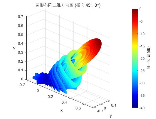
- A 3D pattern over the visible hemisphere, with radius and color in normalized dB
- A four-angle beam scanning demo arranged in a 2 by 2 subplot grid
The script also verifies the peak direction by comparing the designed (theta0, phi0) against the direction the computed pattern actually peaks at, and it reports directivity D0 in dBi using trapezoidal integration over the upper half space.
The Complete MATLAB Script
Copy the code below into MATLAB and run it. For a different array or scan angle, only sections 1 and 2 need editing.
%  Circular planar phased-array antenna design -- beam scanning / 2D and 3D patterns / element coordinates
%  ------------------------------------------------------------------------
%  Array   : concentric-ring planar array in the x-y plane, boresight +z, uniform amplitude excitation
%            center element + Nring concentric rings; ring radius spacing dr
%            elements per ring follow the arc spacing ~dr: Nm = round(2*pi*rm/dr)
%            odd rings are offset by half an angular step, improving nearest-neighbor
%            uniformity and lowering periodic grating lobes
%  Scanning: change only the theta0 / phi0 parameters to steer the beam anywhere
%  Outputs : Fig 1 element coordinates and ring topology (color = excitation phase)
%            Fig 2 2D pattern (scan-plane / principal-plane cuts + u-v plane contour)
%            Fig 3 3D pattern (visible hemisphere, radius and color = normalized dB)
%            Fig 4 multi-angle beam scanning demo
%            element_coord_circ.csv (ring id + element coordinates + excitation amplitude/phase)
%  Notes   : a circular aperture has no edge corners, so the pattern is rotationally
%            symmetric with uniform sidelobes; for the same aperture and gain, a circular
%            array saves the four corner elements a rectangular grid would need
%  Assumes : isotropic elements, mutual coupling neglected; MATLAB R2016b or later
%% ========================================================================
clear; clc; close all;
%% 1. Basic array parameters (editable)
c      = 3e8;              % speed of light (m/s)
f      = 10e9;             % operating frequency (Hz)
lambda = c/f;              % wavelength (m)
k      = 2*pi/lambda;      % wavenumber
Nring  = 10;               % number of concentric rings (excluding the center element)
dr     = lambda/2;         % ring radius spacing (also the nominal arc spacing on a ring)
stagger = true;            % offset odd rings by half an angular step (true/false)
%% 2. Scan angle input (change these two angles to steer)
theta0 = 45;               % scan angle theta0 (deg): measured from the +z axis, 0 to 90
phi0   = 0;                % scan angle phi0 (deg): measured from the +x axis, 0 to 360
u0 = sind(theta0)*cosd(phi0);          % pointing direction in u-v space
v0 = sind(theta0)*sind(phi0);
%% 3. Element coordinates (origin at the array center): center element + each concentric ring
xe = 0;  ye = 0;  ringId = 0;          % center element
Ne_ring = zeros(Nring,1);              % element count per ring
for m = 1:Nring
    rm = m*dr;
    nm = round(2*pi*rm/dr);            % elements on this ring, keeping arc spacing ~dr
    Ne_ring(m) = nm;
    ang = (0:nm-1).' * 2*pi/nm;
    if stagger && mod(m,2)==1
        ang = ang + pi/nm;             % offset odd rings by half an angular step
    end
    xe = [xe; rm*cos(ang)];
    ye = [ye; rm*sin(ang)];
    ringId = [ringId; m*ones(nm,1)];
end
Ne = numel(xe);                        % total number of elements
R  = Nring*dr;                         % aperture radius
fprintf('Array: %d rings + center element, %d elements total, aperture radius %.3f m = %.2f lambda\n', ...
        Nring, Ne, R, R/lambda);
% nearest-neighbor spacing self-check
dxs = xe - xe.';  dys = ye - ye.';
dd = hypot(dxs, dys);  dd(1:Ne+1:end) = NaN;
fprintf('Nearest-neighbor element spacing: min %.3f lambda, max %.3f lambda\n', min(dd(:),[],'omitnan')/lambda, ...
        max(dd(:),[],'omitnan')/lambda);
% Excitation: uniform amplitude + scan phase taper w = exp(-jk(x*u0 + y*v0))
% For lower sidelobes add a radial amplitude taper, e.g. w = w .* (1 - (r/R).^2).^p
w = exp(-1j*k*(xe*u0 + ye*v0));
Amax = Ne;                             % array factor peak for uniform excitation
%% 4. Numerical grating-lobe check (works for any layout: find high-level plateaus outside the main lobe on the u-v grid)
Ng = 301;
ug = linspace(-1, 1, Ng);
[UG, VG] = meshgrid(ug, ug);
vis = UG.^2 + VG.^2 <= 1;             % visible region
AFg0 = af_uv(UG, VG, w, xe, ye, k);
dBg0 = 20*log10(abs(AFg0)/Amax + eps);
dBg0(~vis) = NaN;
rML  = lambda/(2*R);                   % order of magnitude of the main-lobe half width (u-v space)
away = hypot(UG-u0, VG-v0) > 2*rML;    % exclude the main-lobe neighborhood
SLL  = max(dBg0(away & vis));
if SLL > -10
    fprintf('Warning: highest level outside the main lobe is %.1f dB, a grating lobe may exist!\n', SLL);
else
    fprintf('Grating-lobe check: no grating lobe in the visible region (highest level outside the main lobe %.1f dB)\n', SLL);
end
%% 5. 2D pattern: angular cuts + u-v plane contour
th  = (-90:0.1:90).';                  % cut angle sweep
AF1 = af_uv(sind(th)*cosd(phi0), sind(th)*sind(phi0), w, xe, ye, k);  % scan plane
AF2 = af_uv(sind(th), zeros(size(th)),             w, xe, ye, k);  % phi=0 principal plane
AF3 = af_uv(zeros(size(th)), sind(th),             w, xe, ye, k);  % phi=90 principal plane
F1 = 20*log10(abs(AF1)/Amax + eps);
F2 = 20*log10(abs(AF2)/Amax + eps);
F3 = 20*log10(abs(AF3)/Amax + eps);
figure('Name','2D pattern','Color','w');
subplot(2,1,1);
plot(th, F1, 'b', th, F2, 'r--', th, F3, 'g-.', 'LineWidth', 1.1); grid on;
axis([-90 90 -40 2]); hold on;
plot([theta0 theta0], [-40 2], 'k:', 'LineWidth', 1);
xlabel('\theta (deg)'); ylabel('normalized |E| (dB)');
legend(sprintf('scan plane \\phi=%g\\circ', phi0), ...
       '\phi=0\circ (x-z plane)', '\phi=90\circ (y-z plane)', 'Location','southwest');
title(sprintf('Circular array 2D cut pattern (pointing \\theta_0,\\phi_0 = %g\\circ, %g\\circ)', ...
      theta0, phi0));
subplot(2,1,2);
plot_uvmap(ug, dBg0, u0, v0, 'u-v plane pattern (white area is invisible space)');
% peak direction verification
[~, im] = max(AFg0(:).*vis(:));
th_pk = asind(hypot(UG(im), VG(im)));
ph_pk = atan2d(VG(im), UG(im));
fprintf('Designed pointing (theta0, phi0) = (%g deg, %g deg), actual peak direction = (%.2f deg, %.2f deg)\n', ...
        theta0, phi0, th_pk, ph_pk);
%% 6. 3D pattern (visible hemisphere)
th3 = 0:1:90;  ph3 = 0:1:360;
[TH3, PH3] = meshgrid(th3, ph3);
U3 = sind(TH3).*cosd(PH3);   V3 = sind(TH3).*sind(PH3);
AF3d = af_uv(U3, V3, w, xe, ye, k);
dB3 = max(20*log10(abs(AF3d)/Amax + eps), -40);
r3  = (dB3 + 40)/40;                   % normalized radius 0 to 1
figure('Name','3D pattern','Color','w');
surf(r3.*U3, r3.*V3, r3.*cosd(TH3), dB3, 'EdgeColor','none');
hold on;
plot3([0 u0], [0 v0], [0 cosd(theta0)], 'r-', 'LineWidth', 2);   % pointing marker
colormap(gca, jet); cb = colorbar; cb.Label.String = 'normalized |E| (dB)';
axis equal; view(45, 25);
xlabel('x'); ylabel('y'); zlabel('z');
title(sprintf('Circular array 3D pattern (pointing %g\\circ, %g\\circ)', theta0, phi0));
% Directivity (trapezoidal integration over the upper half space; symmetric radiation below doubles it)
P = abs(AF3d).^2 .* sin(deg2rad(TH3));    % integrand (with the sin(theta) weight)
Pint = trapz(deg2rad(th3), trapz(deg2rad(ph3), P, 1), 2);
D0 = 4*pi*Amax^2 / (2*Pint);
fprintf('Directivity D0 = %.2f dBi\n', 10*log10(D0));
%% 7. Element coordinate plot (with ring topology, color = excitation phase)
pha = angle(w)*180/pi;
figure('Name','Element coordinates','Color','w');
thc = linspace(0, 2*pi, 181);
hold on;
for m = 1:Nring
    plot(m*dr*cos(thc), m*dr*sin(thc), '-', 'Color', [0.75 0.75 0.75], 'LineWidth', 0.6);
end
scatter(xe, ye, 42, pha, 'filled');
colormap(gca, jet); cb = colorbar; cb.Label.String = 'excitation phase (deg)';
axis equal; grid on;
xlabel('x (m)'); ylabel('y (m)');
title(sprintf('Circular array element coordinates (%d rings + center, %d elements, scanning to %g\\circ, %g\\circ)', ...
      Nring, Ne, theta0, phi0));
%% 8. Multi-angle beam scanning demo
scan_list = [0 0; 30 0; 30 45; 60 45];          % each row is [theta0, phi0]
figure('Name','Beam scanning demo','Color','w');
for si = 1:size(scan_list,1)
    ts = scan_list(si,1);  ps = scan_list(si,2);
    us = sind(ts)*cosd(ps);  vs = sind(ts)*sind(ps);
    Ws = exp(-1j*k*(xe*us + ye*vs));
    AFs = af_uv(UG, VG, Ws, xe, ye, k);
    dBs = 20*log10(abs(AFs)/Amax + eps);
    dBs(~vis) = NaN;
    subplot(2,2,si);
    plot_uvmap(ug, dBs, us, vs, sprintf('scan (%g\\circ, %g\\circ)', ts, ps));
end
%% 9. Export element coordinates and excitation (CSV, sorted by ring: center element, then ring 1, ...)
T = table((1:Ne).', ringId, xe, ye, abs(w), angle(w)*180/pi, ...
    'VariableNames', {'Element','Ring','X_m','Y_m','Amp_lin','Phase_deg'});
writetable(T, 'element_coord_circ.csv');
fprintf('Element coordinates/excitation exported: element_coord_circ.csv (%d elements)\n', Ne);
%% ---------------- local functions ----------------
function AF = af_uv(U, V, w, xe, ye, k)
% Compute the array factor on a u-v grid (U and V the same size)
% AF(u,v) = sum_i w_i exp[jk(x_i u + y_i v)] (accumulated element by element, valid for any layout)
Uc = U(:);  Vc = V(:);
AF = zeros(numel(Uc), 1);
for i = 1:numel(xe)
    AF = AF + w(i) * exp(1j*k*(xe(i)*Uc + ye(i)*Vc));
end
AF = reshape(AF, size(U));
end
function plot_uvmap(ug, dB, u0, v0, ttl)
% u-v plane pattern: visible-region circle + beam pointing marker, common color scale [-40, 0] dB
imagesc(ug, ug, dB); axis xy; hold on;
thc = linspace(0, 2*pi, 181);
plot(cos(thc), sin(thc), 'w-', 'LineWidth', 0.8);     % visible-region boundary
plot(u0, v0, 'r+', 'MarkerSize', 10, 'LineWidth', 2); % beam pointing
colormap(gca, jet); caxis([-40 0]); colorbar;
xlim([-1.05 1.05]); ylim([-1.05 1.05]);
xlabel('u = sin\theta cos\phi'); ylabel('v = sin\theta sin\phi');
title(ttl);
end
Run Results
Have questions about this article? Feel free to contact us at [email protected] — we’re happy to help!
Frequently Asked Questions
What is a circular phased array antenna?
A circular phased array places radiating elements on concentric rings around a center element rather than on a rectangular grid. Because the aperture has no corners, the pattern stays rotationally symmetric and sidelobes remain uniform as the beam rotates. It also uses fewer elements than a rectangular grid of the same aperture.
How do you steer the beam in this MATLAB script?
Change two variables: theta0 and phi0. Everything else is derived. The script converts those angles into u-v space and applies a progressive phase taper, w = exp(-jk(x*u0 + y*v0)), across the aperture. Every element keeps the same amplitude, so only the phase distribution changes as the beam moves.
Why are the odd rings offset by half an angular step?
Offsetting odd rings staggers the elements so no two rings line up radially. That evens out the nearest-neighbor spacing across the aperture and breaks the periodic structure that would otherwise produce grating lobes. Set the stagger flag to false to compare the two layouts and see the difference in the pattern.
How many elements does the default circular array use?
With 10 rings at half-wavelength spacing, each ring holds round(2*pi*m) elements, which totals 346 across the rings plus 1 center element, so 347 elements. The aperture radius is 5 wavelengths. Changing Nring or dr changes both the element count and the aperture size proportionally.
How does the script check for grating lobes?
It samples the array factor on a 301 by 301 grid in u-v space, keeps only the visible region where u^2 + v^2 is at most 1, masks out the main lobe, and takes the highest remaining level. Above -10 dB it warns of a possible grating lobe; below that it reports a clean region.
About Aomway
Aomway is a technology company specializing in drone and FPV equipment, publishing in-depth analyses of motor control, embedded hardware, and open-source robotics projects. With over 15 years of industry experience, Aomway covers the full spectrum from flight controllers and FPV goggles to thermal imaging cameras and long-range datalinks for the global drone community.